Methods for Generating Random Variables

1. Sampling from a finite population

#toss some coins
sample(0:1, size = 10, replace = TRUE)

#choose some lottery numbers
sample(1:100, size = 6, replace = FALSE)

#permuation of letters a-z
sample(letters)

#sample from a multinomial distribution
x <- sample(1:3, size = 100, replace = TRUE, prob = c(.2, .3, .5))
table(x)

2. Inverse transform method, continuous case

n <- 1000
u <- runif(n)
x <- u^(1/3)

hist(x, prob = TRUE, main = bquote(f(x)==3*x^2)) #density histogram of sample

y <- seq(0, 1, .01)
lines(y, 3*y^2)    #density curve f(x)

4. Two point distribution

n <- 1000
p <- 0.4
u <- runif(n)
x <- as.integer(u > 0.6)   #(u > 0.6) is a logical vector

mean(x) # 1000*0.4
var(x) # 1000*0.4*0.6

5. Geometric distribution

n <- 1000
p <- 0.3
u <- runif(n)

x <- floor(log(u)/log(1-p)) + 1
y <- rgeom(n,p)

par(mfrow = c(1,2))
barplot(table(x))
barplot(table(y))

7. Acceptance-rejection method

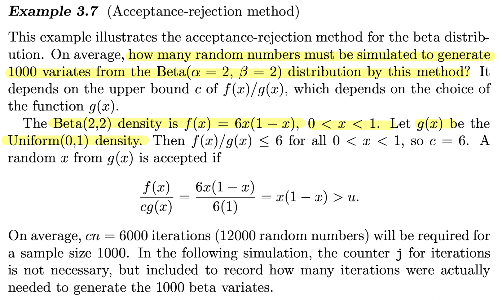
n <- 1000
k <- 0      #counter for accepted
j <- 0      #iterations
y <- numeric(n) # 길이 1000 비어있는 벡터

while (k < n) {
  u <- runif(1)
  j <- j + 1
  x <- runif(1)  #random variate from g
  if (x * (1-x) > u) {
    #we accept x
    k <- k + 1
    y[k] <- x
  }
}

j

# 위 예시는 C = 6 일 때,
# C를 가장 빡빡하게 잡으면 조금만 돌리고도 1000개 난수 생성 가능, 이때 C = 3/2
# qqplot으로 두 개가 같은 분포를 따르는지, 직선 확인

#compare empirical and theoretical percentiles
p <- seq(.1, .9, .1)

Qhat <- quantile(y, p)   #quantiles of sample
Q <- qbeta(p, 2, 2)      #theoretical quantiles

se <- sqrt(p * (1-p) / (n * dbeta(Q, 2, 2)^2)) #see Ch. 2  # 표준오차
round(rbind(Qhat, Q, se), 3)

8. Transformation method, Beta distribution

# 5
n <- 1000
a <- 3
b <- 2

u <- rgamma(n, shape=a, rate=1)
v <- rgamma(n, shape=b, rate=1)

x <- u / (u + v)
q <- qbeta(ppoints(n), a, b)

# Q-Q plot은 두 확률 분포를 그것들의 quantiles를 그려넣음으로써 비교 하는 것이다.
qqplot(q, x, cex=0.25, xlab="Beta(3, 2)", ylab="Sample")
abline(0, 1)

10. Chi-square

n <- 1000
nu <- 2
X <- matrix(rnorm(n*nu), n, nu)^2 #matrix of sq. normals

#sum the squared normals across each row: method 1
y <- rowSums(X)
#method 2
y <- apply(X, MARGIN=1, FUN=sum)  #a vector length n

mean(y)
mean(y^2)

11. Convolutions and mixtures

n <- 1000
x1 <- rgamma(n, 2, 2)
x2 <- rgamma(n, 2, 4)

s <- x1 + x2              #the convolution

u <- runif(n)
k <- as.integer(u > 0.5)  #vector of 0's and 1's
x <- k * x1 + (1-k) * x2  #the mixture

par(mfcol=c(1,2))         #two graphs per page
hist(s, prob=TRUE, xlim=c(0,5), ylim=c(0,1))
hist(x, prob=TRUE, xlim=c(0,5), ylim=c(0,1))
par(mfcol=c(1,1))         #restore display

12. Mixture of several gamma distributions

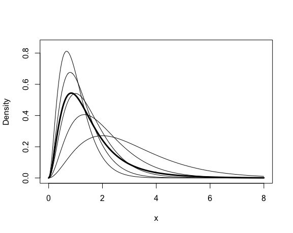
# density estimates are plotted
# X_k ~ Gamma(3,1/k)
# p_k = k/15, k=1,2,3,4,5
n <- 5000
k <- sample(1:5, size=n, replace=TRUE, prob=(1:5)/15)
rate <- 1/k
x <- rgamma(n, shape=3, rate=rate)

#plot the density of the mixture
#with the densities of the components
plot(density(x), xlim=c(0,40), ylim=c(0,.3),
     lwd=3, xlab="x", main="")
for (i in 1:5)
  lines(density(rgamma(n, 3, 1/i)))

n <- 5000
p <- c(.1,.2,.2,.3,.2)
lambda <- c(1,1.5,2,2.5,3)
k <- sample(1:5, size=n, replace=TRUE, prob=p)
rate <- lambda[k]
x <- rgamma(n, shape=3, rate=rate)

14. Plot density of mixture

f <- function(x, lambda, theta) {
  #density of the mixture at the point x
  sum(dgamma(x, 3, lambda) * theta)
}

p <- c(.1,.2,.2,.3,.2)
lambda <- c(1,1.5,2,2.5,3)

x <- seq(0, 8, length=200)
dim(x) <- length(x)  #need for apply

#compute density of the mixture f(x) along x
y <- apply(x, 1, f, lambda=lambda, theta=p)

#plot the density of the mixture
plot(x, y, type="l", ylim=c(0,.85), lwd=3, ylab="Density")

for (j in 1:5) {
  #add the j-th gamma density to the plot
  y <- apply(x, 1, dgamma, shape=3, rate=lambda[j])
  lines(x, y)
}

15. Poisson-Gamma mixture

#generate a Poisson-Gamma mixture
n <- 1000
r <- 4
beta <- 3
lambda <- rgamma(n, r, beta) #lambda is random

#now supply the sample of lambda's as the Poisson mean
x <- rpois(n, lambda)        #the mixture

#compare with negative binomial
mix <- tabulate(x+1) / n
negbin <- round(dnbinom(0:max(x), r, beta/(1+beta)), 3)
se <- sqrt(negbin * (1 - negbin) / n)

round(rbind(mix, negbin, se), 3)