AI-900 정리노트 - Overview

파란색 글자에 마우스를 올리면 설명이 나옵니다

Machine learning

Supervised machine learning

• The training data includes both feature and known label values

Regression

• label predicted by the model is numeric form

Classification

• label represents a categorization or class

EX

1. Binary classification
2. Multiclass classification

Unsupervised machine learning

• the training data consists of only the feature values without known labels

Clustering

• Group similar flowers based on size, ...
• Identify groups of similar customers with ...

---

Regression

1. Split Data: Randomly divide your data into a training set (for model fitting) and a validation set (for testing).
2. Train Model: Use an appropriate algorithm (e.g., linear regression for regression tasks) to train the model on the training data.
3. Validate Model: Use the trained model to predict outcomes for the validation set.
4. Evaluate Performance: Compare the model's predictions against the actual known values in the validation set and calculate a performance metric (e.g., accuracy, error rate) to assess the model's effectiveness.

Regression evaluation metrics

• Mean Absolute Error (MAE): The average of the absolute differences between predicted and actual values.
• Mean Squared Error (MSE): The average of the squared differences between predicted and actual values. Penalizes larger errors more heavily due to squaring. The unit is the square of the original label's unit.
• Root Mean Squared Error (RMSE): The square root of the MSE. Returns the error metric to the original unit of the label, making it more interpretable than MSE while still penalizing larger errors.

coefficient of determination

The Coefficient of Determination (R² or R-Squared) measures the proportion of the variance in the dependent variable (e.g., actual sales) that is predictable from the independent variable(s) in a regression model.

Unlike metrics that only compare prediction errors, R² considers the inherent random variance in the data. It compares the variance of the model's errors to the total variance of the actual data.

Calculation:

$R^2 = 1 - \frac{\sum(y - \hat{y})^2}{\sum(y - \bar{y})^2}$

Where:

• $y$ = Actual value
• $\hat{y}$ = Predicted value
• $\bar{y}$ = Mean of the actual values
• $\sum(y - \hat{y})^2$ = Sum of squared errors (variance unexplained by the model)
• $\sum(y - \bar{y})^2$ = Total sum of squares (total variance in the data)

Interpretation:

• R² ranges from 0 to 1.
• A value closer to 1 indicates that a larger proportion of the variance in the data is explained by the model, suggesting a better fit.
• A value of 0 means the model explains none of the variance.
• A value of 1 means the model explains all the variance.

For example, an R² of 0.95 means the model explains 95% of the variance observed in the validation data.

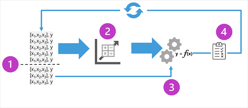
Iterative training

• Iterative process to repeatedely train and evaluate a model

How?

• Feature selection, Preparation
• Algorithm selection
• Algorithm parameters

---

Binary classification

• Calculate probability values for class assignment, Evaluation metrics of model is comparing the predicted classes to the actual classes

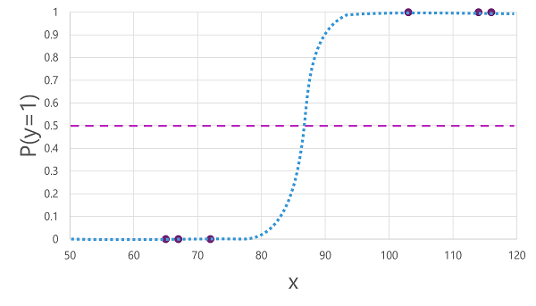
How to train the model

• Use an algorithm to fit the training data to a function that calculates the probability of the class label being true

For example,

• Probability of a patient having a diabetes is 0.7
• Then patient who does not have a diabetes will be 0.3

So then

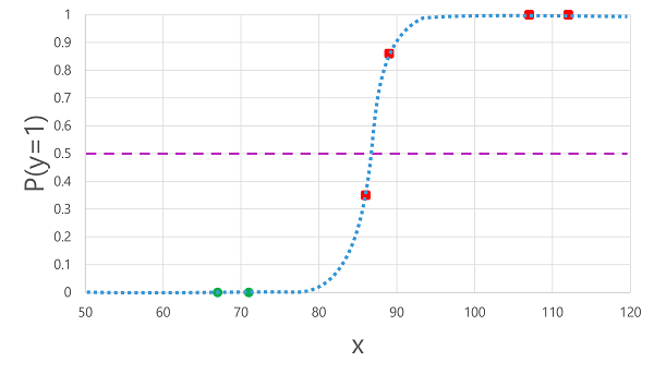
• Can use logistic regression, which derives a sigmod function with values between 0 and 1
  
  

Evaluation metrics

• Create a matrix of correct and incorrect predictions for each possible label
  
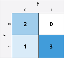
• ŷ=0 and y=0: True negatives (TN)
• ŷ=1 and y=0: False positives (FP)
  • Predicted as True, but actually False
• ŷ=0 and y=1: False negatives (FN)
  • Predicted as False, but actually True
• ŷ=1 and y=1: True positives (TP)

Accuracy

• Caluated as below

  (TN+TP) ÷ (TN+FN+FP+TP)

Recall

• Proportion of positive cases that the model identified correctly

  (TP) / (TP + FN)

F-1 Score

• overall metrics that combined recall and precision

  (2 Precision recall) / (Precision + recall)

Area Under the Cover ( AUC )

• We can calcalulate FPR ( False positive rate )
  • Means How many of them is Positive but actually negative

    FPR = FP / (FP + TN)

• And can make graph down below
  
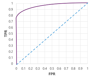
• This is the graph of TPR and FPR while changing Threshhold called Receiver Operating Characteristic Curve ( ROC Curve )
• Idealy, the top-left most position of graph is the best
  • Lowest FPR, and Highst TPR

AUC is the area of ROC graph which has a value of 0.0 ~ 1.0

• Higher auc means it has best performance at predict binary result

---

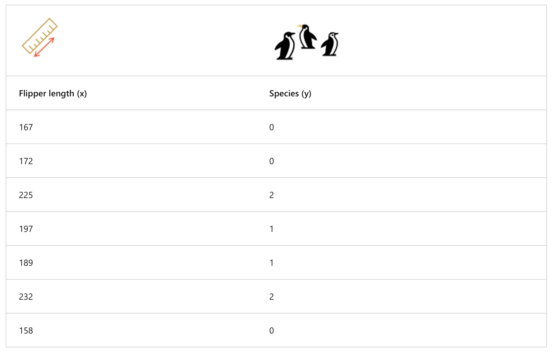
Multiclass classification

• Calculate the probaility of values for multiple class labels

Example, Decide penguin species with height of them

RAW DATA

• There is algorithms we can use

One-vs-Rest (OvR) algorithms

• Train a binary classification for each class
• Each function calculates the probability of the observation being a specific flass compared to other class

  $f^0(x) = P(y=0 | x)$
  $f^1(x) = P(y=1 | x)$
  $f^2(x) = P(y=2 | x)$

Multimominal algorithms

• Single function which produce multi-valued output.
• Output is the vector that contains the probability distribution of all possible classes

  $f(x) =[P(y=0|x), P(y=1|x), P(y=2|x)]$

Evaluate the model

• Calculate aggregate metrics that take all classes into account
  
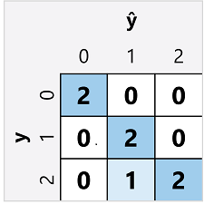
• To calculate the accuracy, use total of the TP, TN, FP, FN

  Overall accuracy = (13+6)÷(13+6+1+1) = 0.90
  Overall recall = 6÷(6+1) = 0.86
  Overall precision = 6÷(6+1) = 0.86

F-1 score

(2x0.86x0.86)÷(0.86+0.86)

---

Clustering

• Unsupervised machine learning in which observations are grouped into clusters based on similiarities in their data values or features.

Example: grouping a flower with numbers of petals and leaves

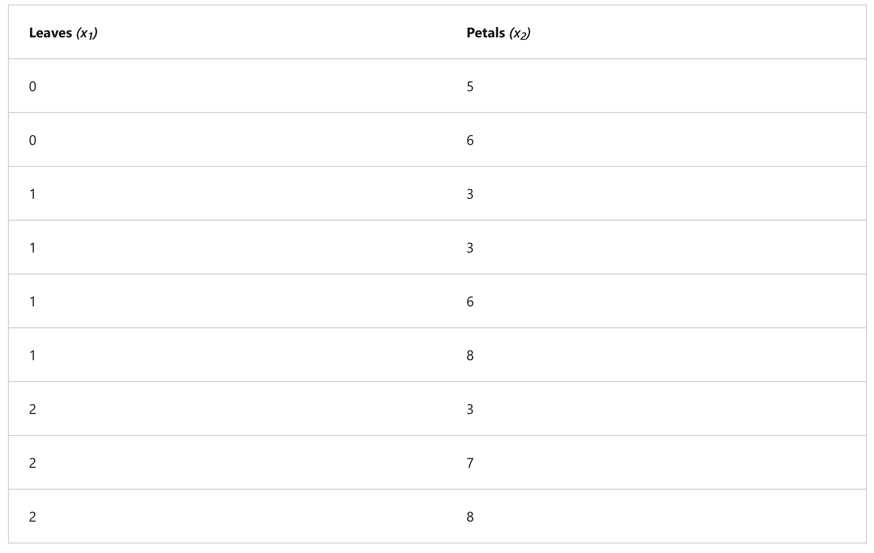
Training data

1. Draw 2-coordinate with the features
2. Decide how many clusters to group the flowers ( call this k ), k points are plotted at random coordinates and they're called centroids
3. Each data point is assigned to its nearest centroid
4. Each centroid is moved to the center of the data points assigned to it based on the mean distance between the points
5. After the centroid is moved, data points can be reassigned to clusters based on the new closest centroid
6. 4, 5 steps are repeated until the clusters become stable or maximum iteration count

Evaluate the clustered model

Average distance to cluster center : How close on average, each point in cluster is to the centroid of the cluster

Average distance to other cluster : How close on average, each point in the cluster is to the centroid of all other clusters

Maximum distance to cluster center : Tue furthest distance between a point in the cluster and its centroid

Silhouette Score: A value between -1 and 1 that summarizes how similar a data point is to its own cluster compared to other clusters. It measures the ratio of intra-cluster distance (distance to points in the same cluster) and inter-cluster distance (distance to points in the nearest neighboring cluster).

• Example Interpretations:

  • A score close to +1 indicates that the data point is well-clustered. It's far from neighboring clusters and close to points in its own cluster. This is the ideal scenario.
  • A score close to 0 suggests the data point is near the boundary between two clusters. Its distance to its own cluster and the nearest neighboring cluster is similar.
  • A score close to -1 indicates that the data point might be misclassified. It's closer, on average, to points in a neighboring cluster than to points in its assigned cluster.

  ---

  Deep learning

• Advanced form of machine learning that tries to emulate the way human learns.

• Creation of artificial nueral network that simulate electrochemical activity in biological neurons by using mathematical functions

HOW?

• Artificial neural networks are made up of multiple layers of neurons
  • deeply nested function
  • DNN / Deep Neural Network
• Fitting training data to a function that can predict a label
  • A neural network is composed of multiple layers, where each layer applies a function to the values (x) received from the previous one. This structure, where one layer's output becomes the next layer's input, resembles a nested function (or function composition), allowing the entire network to compute the output value (y) from the initial input data (x).

Example : Deep learning Classification

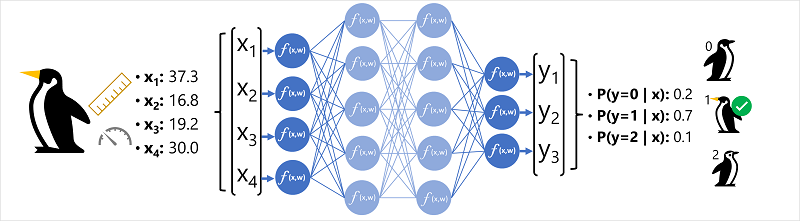
• Input features (x vector, e.g., [37.3, 16.8, 19.2, 30.0]) are fed into the network.
• Data flows through layers where neurons compute weighted sums and apply activation functions.
• The final output layer uses a function like softmax to produce class probabilities (e.g., [0.2, 0.7, 0.1]).
• The class with the highest probability (here, 0.7 for class 1, Gentoo) is the prediction.

How does it works?

1. Input training features into the network.
2. Apply initial random weights and process data through layers.
3. Generate output predictions ($\hat{y}$).
4. Calculate loss by comparing predictions ($\hat{y}$) with actual values ($y$) using a loss function.
5. Use an optimizer (e.g., gradient descent) to determine how to adjust weights to minimize loss.
6. Backpropagate the weight adjustments through the network.
7. Repeat the process over multiple epochs until the model achieves acceptable accuracy.

---

Transformer

• Trained with large volume of text, enabling them to represent the semantic relationship between words and use those relationship to determine probable sequences of text that make sense

How it works

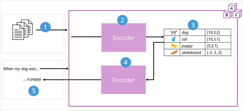
1. The model is trained using large volumes of natural language text, often sourced from the internet.
2. Text sequences are broken into smaller units called tokens (similar to words).
3. An 'encoder' processes these tokens using an 'attention' mechanism to identify relationships and context between them.
4. The encoder produces 'embeddings', which are numerical vectors representing the semantic meaning and attributes of the tokens.
5. A 'decoder' takes new input tokens and uses the embeddings generated by the encoder to create appropriate natural language output.
6. For instance, given "When my dog was", the model uses attention and embeddings to predict a likely completion like "a puppy".

Tokenization

• The first step in training a transformer model
• decompose the training text into token

- I (1)
- heard (2)
- a (3)
- dog (4)
- bark (5)
- loudly (6)
- at (7)
- ("a" is already tokenized as 3)
- cat (8)

Embedding

1. Problem: Just giving words unique ID numbers (like in a dictionary index) doesn't tell us anything about their meaning or how they relate to other words.
2. Solution: We use embeddings. Think of embeddings as rich, numerical descriptions for each word, stored as a list of numbers called a vector (e.g., [10, 3, 1]).
3. Meaning in Numbers: Each number in the vector represents some aspect of the word's meaning or how it's typically used. The model figures out these numbers during training by looking at which words often appear together or in similar situations.
4. Vectors as Locations: You can imagine these vectors as coordinates pointing to a specific location in a multi-dimensional "meaning space". Each number in the vector acts like a direction (e.g., how "positive/negative", how "abstract/concrete", etc.).
5. Relationships: Words with similar meanings or uses will have vectors pointing to nearby locations in this "meaning space". This allows the model to understand relationships between words numerically.

- 4 ("dog"): [10,3,2]
- 8 ("cat"): [10,3,1]
- 9 ("puppy"): [5,2,1]
- 10 ("skateboard"): [-3,3,2]

Attention

1. Both the encoder and decoder parts of a transformer model contain layers, including important ones called attention layers.
2. Attention is a technique the model uses to analyze text and figure out how strongly different words in a sequence influence each other.
3. Self-attention specifically looks at how the surrounding words (the context) affect the meaning of one particular word within that sequence.
4. In the encoder, self-attention helps create word embeddings (numerical representations) that are sensitive to this context.
5. This means the same word can get different embeddings depending on how it's used. For example, "bark" means one thing (and gets one embedding) in "the bark of a tree" and something else (with a different embedding) in "I heard a dog bark".

HOW IT WORKS?

1. A sequence of token embeddings is fed into the attention layer. Each token is represented as a vector of numeric values.
2. The goal in a decoder is to predict the next token in the sequence, which will also be a vector that aligns to an embedding in the model’s vocabulary.
3. The attention layer evaluates the sequence so far and assigns weights to each token to represent their relative influence on the next token.
4. The weights can be used to compute a new vector for the next token with an attention score. Multi-head attention uses different elements in the embeddings to calculate multiple alternative tokens.
5. A fully connected neural network uses the scores in the calculated vectors to predict the most probable token from the entire vocabulary.
6. The predicted output is appended to the sequence so far, which is used as the input for the next iteration.

Large language models like GPT-4 are trained on vast amounts of data using complex networks and attention mechanisms to predict probable word sequences, enabling them to generate coherent, human-like text completions for prompts by leveraging learned statistical patterns rather than possessing actual knowledge or intelligence.

---

Azure

Feature

• Prebuild & Ready to use
• Accessed through API
• Available and secure on Azure

How to use

• Create a Azure AI Service Resource