모델 개발 개요(Overview)

2022-08-10 ~ 2022-08-12 기간동안 대한산업공학회에서 진행하는 Field Camp에 참여했다. 주제는 건강검진 정보를 활용하여 흡연예측 모델을 만드는 것이었다. 총 9명의 팀원들과 같이 활동을 했고 여기에서 내가 맡은 파트는 모델 개발이었다.

I participated in the Field Camp held by the Korea Industrial Engineering Association during the 2022-08-10 to 2022-08-12. The theme was to create a smoking prediction model using health examination information. I worked with 9 team members, and my part was model development.

EDA(Exploratory Data Analysis)

데이터 정보(About Data)

열 개수(Number of columns): 29

열 구성요소(The elements in the columns of the data are as follows):

• 수치형 자료(Numerical data)
  AGE, HEIGHT, WEIGHT, WAIST, SIGHT_LEFT, SIGHT_RIGHT, HEAR_LEFT, HEAR_RIGHT, BP_HIGH(수축기 혈압), BP_LWST(이완기 혈압), BLDS(식전혈당), TOT_CHOLE(총 콜레스테롤), TRIGLYCERIDE(트리글리세라이드), HDL_CHOLE(HDL 콜레스테롤), LDL_CHOLE(LDL 콜레스테롤), HMG(혈색소), OLIG_PROTE(요단백), CREATININE(혈청 크레아티닌), SGOT_AST(혈청 지오티 AST), SGOT_ALT(혈청지오티 ALT), GAMMA_GTP
• 범주형 자료(Categorical data)
  ID, SEX, SIDO(거주지), DRK_YN(음주여부), HCHK_OE_INSPEC_YN(구강검진수검여부), CRS_YN(치아우식증 유무), TTR_YN(치석 여부), SMK_STAT(흡연상태)

예시 데이터(Example data):

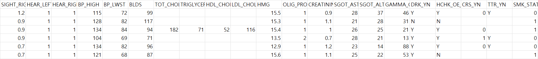
분석에 앞서 SMK_STAT는 0,1,2로 구성되어 있는데 0은 담배를 피지 않음, 1은 담배를 핌, 2는 담배를 피다가 끊음이다. 추후 서술하겠지만 상태 2는 상태 1과 건강상태가 유사하여 1로 취급하여 분석을 진행한다.

Prior to the analysis, SMK_STAT consists of 0, 1, and 2.
0 means not smoking, 1 means smoking, and 2 means quitting smoking. As will be described later, status 2 is similar to status 1, so the analysis is conducted by treating 2 as 1.

간 기능 지표 분석(Analysis of Liver Function Indicators)

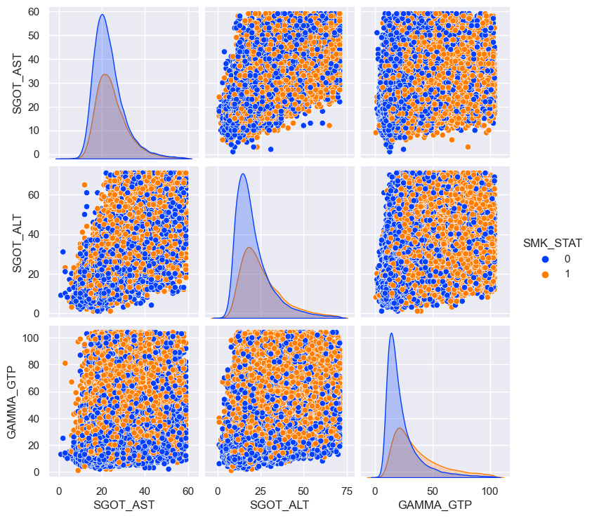
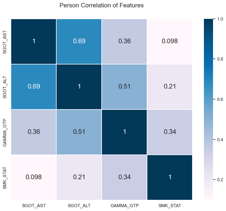
간 기능과 관련된 지표는 감마지티피, 혈청 지오티 ALT/AST 이다. 데이터프레임에서 IQR 범위에 1.5를 곱한 범위 외부의 값을 이상치로 규정하였다. 이후 seaborn을 이용하여 산점도 행렬을 구성하였다. 또한 heatmap을 활용하여 상관계수를 직관적으로 파악하였다.

Indicators associated with liver function are GAMMA_GTP, SGOT ALT/AST. In the data frame, a value outside the range which multiply the IQR range by 1.5 was defined as an outlier. Thereafter, a scatterplot matrix was constructed by using seaborn module. In addition, the correlation coefficient was intuitively shown using heatmap.

코드(Programming Code, Python)

• 이상치 제거 함수(Outliers Removal Function)

liver_col = ['SGOT_AST','SGOT_ALT','GAMMA_GTP','SMK_STAT']
liver_df = raw_smoke[liver_col]

def remove_out(dataframe, remove_col):
    dff = dataframe
    for k in remove_col:
        level_1q = dff[k].quantile(0.25)
        level_3q = dff[k].quantile(0.75)
        IQR = level_3q - level_1q
        rev_range = 3  # 제거 범위 조절 변수
        dff = dff[(dff[k] <= level_3q + (rev_range * IQR)) & (dff[k] >= level_1q - (rev_range * IQR))]
        dff = dff.reset_index(drop=True)
    return dff

liver_df = remove_out(liver_df, liver_col)

• 산점도 행렬(Scatter plot)

import seaborn as sns
sns.pairplot(liver_df,
            diag_kind = 'kde',
            hue = 'SMK_STAT',
            palette= 'bright')

plt.show()

• 상관계수(Correlation coefficient)

colormap = plt.cm.PuBu
plt.figure(figsize=(10, 8))
plt.title("Person Correlation of Features", y = 1.05, size = 15)
sns.heatmap(liver_df.astype(float).corr(), linewidths = 0.1, vmax = 1.0,
            square = True, cmap = colormap, linecolor = "white", annot = True, annot_kws = {"size" : 16})

Output

Scatter plot

Correlation coefficient

Result

1. 담배를 피는 집단에서 SGOT_AST와 GAMMA_GTP 수치가 담배를 피지 않는 집단에 비해 높게 나타난다.

   In the smoking group, SGOT_AST and GAMMA_GTP levels are higher than in the non-smoking group.

2. SGOT_AST, SGOT_ALT, GAMMA_GTP 사이에서는 유의미한 양의 상관관계가 나타난다.

   A significant positive correlation appears between SGOT_AST, SGOT_ALT, and GAMMA_GTP.

고지혈증 관련 지표 분석(Analysis of indicators related to hyperlipidemia)

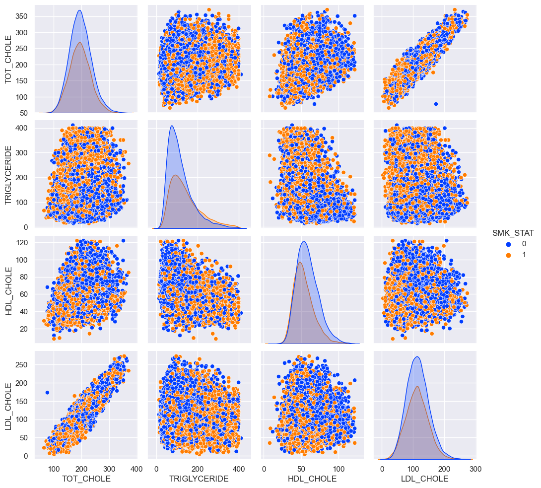
지방이 분해되면서 생기는 콜레스테롤과 중성지방은 고지혈증을 측정하는 가장 강력한 지표이다. 이와 관련된 지표는 TOT_CHOLE, TRIGLYCERIDE(중성지방), HDL_CHOLE, LDL_CHOLE 이다. HDL_CHOLE은 일반적으로 신체에 긍정적 영향을 LDL_CHOLE은 신체에 악영향을 주는 것으로 알려져 있다. 간 기능 지표 분석과 동일한 방식으로 진행하였다. 코드는 거의 유사하기에 생략한다.

Cholesterol and triglycerides produced by the decomposition of fat are the strongest indicators for measuring hyperlipidemia. The related indicators are TOT_CHOLE, TRIGLYCERIDE, HDL_CHOLE, and LDL_CHOLE. HDL_CHOLE is generally known to have a positive effect on the body, and LDL_CHOLE has a negative effect on the body. Analysis was conducted in the same way as the liver function indicators analysis. The programming code is almost similar, so I'll omit it.

Output

Scatter plot

Correlation coefficient

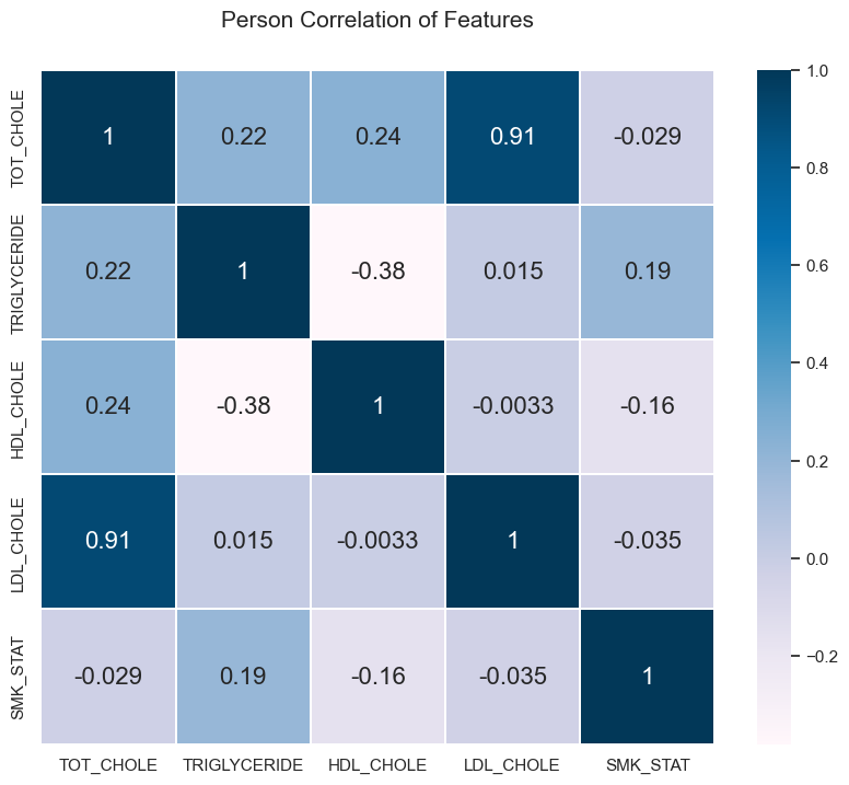
Result

1. 흡연자는 비흡연자에 비해 TRIGLYCERIDE 수치는 높고 HDL_CHOLE 수치는 낮다. 즉 신체에 악영향을 주는 지질의 수치는 높고 긍정적 영향을 주는 지질의 수치는 낮다는 것이다.

   Smokers have a higher TRIGLYCERIDE level and a lower HDL_CHOLE level than non-smokers. In other words, the level of lipids that adversely affect the body is high and the level of lipids that have positive effects is low.

2. 신체의 TOT_CHOLE은 대부분 LDL_CHOLE로 이루어져 있을 가능성이 높음을 상관관계 분석을 통해 알 수 있다.

   It can be seen from correlation analysis that most of the body's TOT_CHOLE is likely to consist of LDL_CHOLE.

3. HDL_CHOLE은 체내의 TRIGLYCERIDE 수치를 낮추는 것에 도움을 줄 가능성이 높다.

   HDL_CHOLE is likely to help lower TRIGLYCERIDE levels in the body.

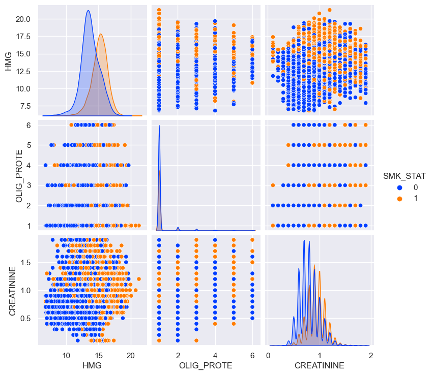
요단백 관련 지표 분석(Analysis of proteinuria related indicators)

요단백과 관련있는 데이터는 HMG(혈색소), OLIG_PROTE(요단백 수치), CREATININE(혈청 크레아티닌) 이다. HMG는 혈액 속 단백질이고 CREATININE는 단백질 대사의 산물으로 단백질의 대사가 얼마나 원활히 이루어지는지를 알 수 있는 척도이다.

Data associated with proteinuria are HMG (hemoglobin), OLIG_PROTE (urinary protein level), and CREATINE (serum creatinine). HMG is a protein in the blood, and CREATININE is a product of protein metabolism and is a measure of how smoothly protein metabolism works.

Output

Scatter plot

Correlation coefficient

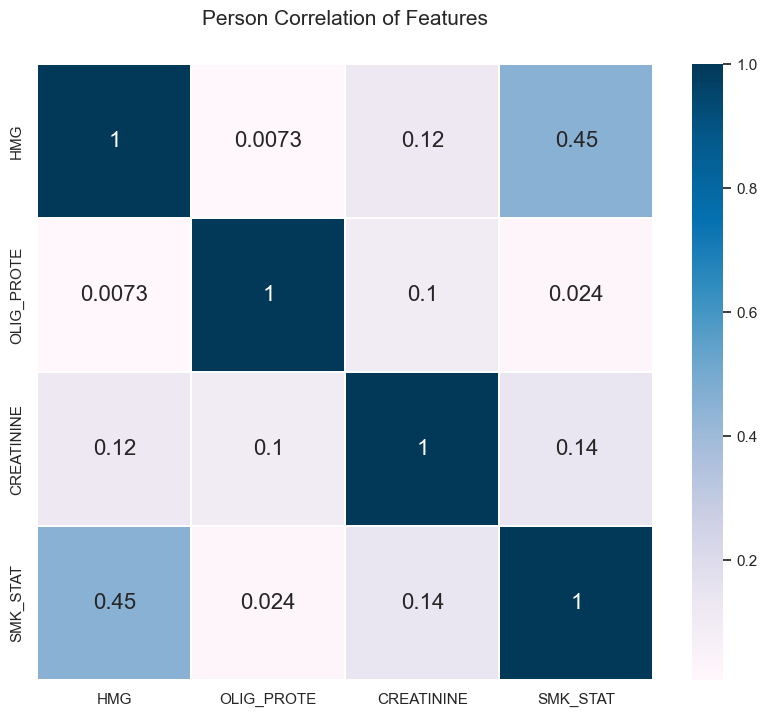
Result

1. OLIG_PROTE(요단백 수치)와 흡연 유무는 거의 관련성이 없다.

   OLIG_PROTE has little relevance to smoking.

2. 흡연 시 HMG 수치와 CREATININE 수치가 높게 유지된다고 볼 수는 있다.

   It can be seen that HMG and CREATINE levels are maintained high when smoking.

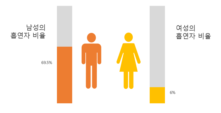
성별과의 관련성(Gender relevance)

SEX와 SMK_STAT는 모두 범주형 데이터 이므로 남,여에서 흡연자 비율을 분석해본다.

Since both SEX and SMK_STAT are categorical data, the proportion of smokers in men and women is analyzed.

Output

남자의 경우 37973명이 흡연자이며 16673명이 비흡연자임이 나타났고 여자의 경우 2998명이 흡연자이며 42356명이 비흡연자로 나타났다. 주의할 점은 담배를 피다가 끊은 사람은 흡연자로 취급하였다.

In the case of men, 37973 were smokers and 16673 were non-smokers, while in the case of women, 2998 were smokers and 42356 were non-smokers. It should be noted that those who quit smoking were treated as smokers.

Result

모델 설계(Model Design)

사용 모듈은 다음과 같다.

# Set up the environment
import warnings
warnings.simplefilter(action='ignore', category=FutureWarning)
import numpy as np
import pandas as pd
import matplotlib.pyplot as plt
import seaborn as sns
sns.set()
from sklearn.model_selection import train_test_split
from sklearn.preprocessing import StandardScaler 
from sklearn.neighbors import KNeighborsClassifier
from sklearn.metrics import classification_report, confusion_matrix
from sklearn.linear_model import LogisticRegression
from sklearn.svm import SVC

데이터 전처리(Data preprocessing)

문자형 데이터를 숫자로 변경(Changing Character Data to Numbers)

# Suppress warnings
pd.options.mode.chained_assignment = None 

# Convert Y -> 1, N -> 0
raw_smoke['DRK_YN'][raw_smoke['DRK_YN'] == 'Y'] = 1
raw_smoke['DRK_YN'][raw_smoke['DRK_YN'] == 'N'] = 0
raw_smoke['HCHK_OE_INSPEC_YN'][raw_smoke['HCHK_OE_INSPEC_YN'] == 'Y'] = 1
raw_smoke['HCHK_OE_INSPEC_YN'][raw_smoke['HCHK_OE_INSPEC_YN'] == 'N'] = 0
raw_smoke['TTR_YN'][raw_smoke['TTR_YN'] == 'Y'] = 1
raw_smoke['TTR_YN'][raw_smoke['TTR_YN'] == 'N'] = 0

# Convert datatype into numeric
raw_smoke = raw_smoke.apply(pd.to_numeric)

결측치 처리(Missing Value Processing)

null값의 비율이 50%를 넘는 데이터 칼럼은 제거하기로 하였음.

It was decided to remove the data column whose null value ratio exceeds 50%.

# null ratio
for col in raw_smoke.columns:
    msg = 'column: {:>10}\t Percent of NaN Value: {:.2f}%'.format(col, 100 * (raw_smoke[col].isnull().sum() / raw_smoke[col].shape[0]))
    print(msg)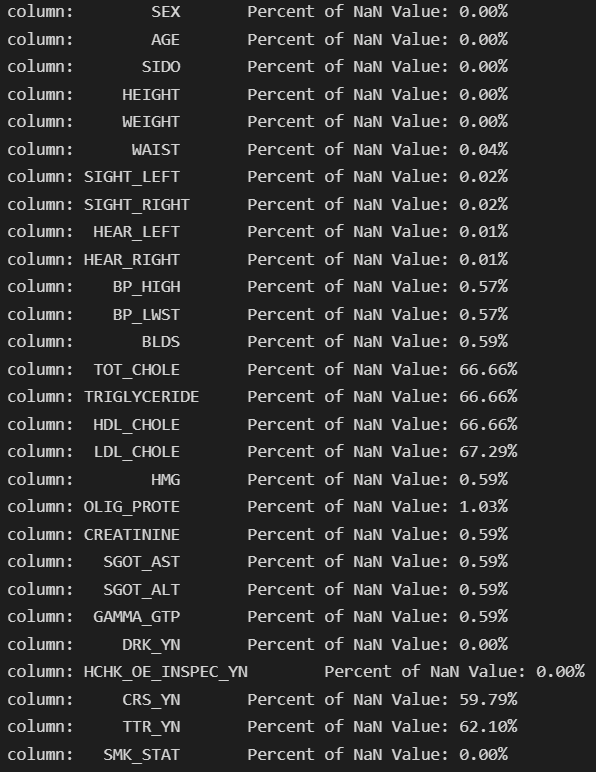

Discard columns which name is TOT_CHOLE , TRIGLYCERIDE , HDL_CHOLE , LDL_CHOLE , CRS_YN , TTR_YN

중앙값 삽입 대신 na가 있는 행를 전부 제거한다. 942개가 삭제 되지만, 이는 전체 데이터셋 크기를 생각하면 무시해도 괜찮은정도이다.

Remove all rows with na instead of median imputation. 942 are deleted, but this is negligible considering the size of the entire dataset.

One-hot Encoding

'SIDO' 변수를 one-hot encoding 한다.
시도코드는 숫자로 이루어져 있지만 numerical variable이 아니라 categorical variable이기 때문이다.

One-hot encoding the 'SIDO' variable.
This is because, even if the 'SIDO' is composed of numbers, it is not numerical variable but categorical variable.

raw_smoke['SIDO'][raw_smoke['SIDO'] == 11] = '서울'
raw_smoke['SIDO'][raw_smoke['SIDO'] == 26] = '부산'
raw_smoke['SIDO'][raw_smoke['SIDO'] == 27] = '대구'
raw_smoke['SIDO'][raw_smoke['SIDO'] == 28] = '인천'
raw_smoke['SIDO'][raw_smoke['SIDO'] == 29] = '광주'
raw_smoke['SIDO'][raw_smoke['SIDO'] == 30] = '대전'
raw_smoke['SIDO'][raw_smoke['SIDO'] == 31] = '울산'
raw_smoke['SIDO'][raw_smoke['SIDO'] == 36] = '세종'
raw_smoke['SIDO'][raw_smoke['SIDO'] == 41] = '경기'
raw_smoke['SIDO'][raw_smoke['SIDO'] == 42] = '강원'
raw_smoke['SIDO'][raw_smoke['SIDO'] == 43] = '충북'
raw_smoke['SIDO'][raw_smoke['SIDO'] == 44] = '충남'
raw_smoke['SIDO'][raw_smoke['SIDO'] == 45] = '전북'
raw_smoke['SIDO'][raw_smoke['SIDO'] == 46] = '전남'
raw_smoke['SIDO'][raw_smoke['SIDO'] == 47] = '경북'
raw_smoke['SIDO'][raw_smoke['SIDO'] == 48] = '경남'
raw_smoke['SIDO'][raw_smoke['SIDO'] == 50] = '제주'

# One-hot encoding
from sklearn.preprocessing import OneHotEncoder
enc = OneHotEncoder(sparse = False) # Create OneHotEncoder object
sido_cat = raw_smoke['SIDO']
sido = enc.fit_transform(sido_cat[:, np.newaxis])
sido_df = pd.DataFrame(sido, columns = enc.get_feature_names()) 

# Replace SIDO with encoded columns
smoke = raw_smoke.drop(['SIDO'], axis = 1)
smoke = smoke.reset_index(drop = True)
smoke = pd.concat([smoke, sido_df], axis = 1)
smoke

이상치 조정(Outlier Processing)

SIGHT_LEFT 와 SIGHT_RIGHT는 실명이 9.9로 표기 되어 있다. 이는 모델을 헷갈리게 할 가능성이 높다. (높을수록 시력이 좋기때문)
그러므로 9.9 를 0 으로 바꿔주고 BLIND_LEFT와 BLIND_RIGHT라는 새로운 column을 만들어 준다.
각각 왼쪽과 오른쪽눈이 실명이라면 1, 그 외 경우 0 이다.

The blindness of SIGHT_LEFT and SIGHT_RIGHT are written as 9.9. This is likely to confuse the model (Generally the higher the better the vision is)
Therefore, it changes 9.9 to 0 and creates new columns called BLIND_LEFT and BLIND_RIGHT.
If each of the left and right eyes are blind, they are 1 and 0 in other cases.

# Initialize
smoke['BLIND_LEFT'] = 0
smoke['BLIND_RIGHT'] = 0

# BLIND column check
smoke['BLIND_LEFT'][smoke['SIGHT_LEFT'] == 9.9] = 1
smoke['BLIND_RIGHT'][smoke['SIGHT_RIGHT'] == 9.9] = 1

# SIGHT column 9.9 -> 0
smoke['SIGHT_LEFT'][smoke['SIGHT_LEFT'] == 9.9] = 0
smoke['SIGHT_RIGHT'][smoke['SIGHT_RIGHT'] == 9.9] = 0

추가 정보 활용하기(Use additional information)

CREATININE, SGOT_AST, SGOT_ALT, GAMMA_GTP 전부 정상, 비정상치가 있다.
각각 이름 뒤 _NORMAL이 붙은 column을 만들어, 정상이면 1, 비정상이면 0 으로 기록한다.

CREATININE, SGOT_AST, SGOT_ALT, and GAMMA_GTP have normal and abnormal value ranges.
Make a column with _NORMAL after each name and record it as 1 if normal and 0 if abnormal.

# Initialize
smoke['CREATININE_NORMAL'] = 0
smoke['SGOT_AST_NORMAL'] = 0
smoke['SGOT_ALT_NORMAL'] = 0
smoke['GAMMA_GTP_NORMAL'] = 0

# NORMAL column
smoke['CREATININE_NORMAL'][(smoke['CREATININE'] >= 0.8) & (smoke['CREATININE'] <= 1.7)] = 1
smoke['SGOT_AST_NORMAL'][(smoke['SGOT_AST'] >= 0) & (smoke['SGOT_AST'] <= 40)] = 1
smoke['SGOT_ALT_NORMAL'][(smoke['SGOT_ALT'] >= 0) & (smoke['SGOT_ALT'] <= 40)] = 1
smoke['GAMMA_GTP_NORMAL'][(smoke['SEX'] == 2) & (smoke['GAMMA_GTP'] >= 8) & (smoke['GAMMA_GTP'] <= 35)] = 1 # 여성
smoke['GAMMA_GTP_NORMAL'][(smoke['SEX'] == 1) & (smoke['GAMMA_GTP'] >= 11) & (smoke['GAMMA_GTP'] <= 63)] = 1  # 남성

SMK_STAT 값이 2인 것 처리하기(Process SMK_STAT value of 2)

SMK_STAT은 0,1,2의 값으로 이루어져 있는데 0은 비흡연자, 1은 흡연자, 2는 담배를 피었다가 끊은 사람을 의미한다. 우리가 흡연 유무를 구분할 Test 테이터 셋에는 비흡연자와 흡연자 둘로만 구성되어 있기에 Train 데이터 셋에서 2를 처리하여야 한다. SMK_STAT이 2인 사람의 수가 상당히 많기에 단순히 drop을 해버리면 정보의 손실이 일어난다. 이러한 이유로 2의 값이 0과 1중 어디에 가까운지 검증하고자 한다.

SMK_STAT consists of values of 0, 1, and 2, where 0 means a non-smoker, 1 means a smoker and 2 means a person who smoked and stopped smoking. Since the Test dataset, which we will distinguish between smoking and non smoking, consists of only non-smokers and smokers, 2 should be processed in the Train dataset. Since number of people whose SMK_STAT value is 2 is quite large, simply dropping causes loss of information. For this reason, we would like to verify whether the value of 2 is close to 0 or 1.

GAMMA_GTP와 HMG 수치에서 흡연자와 비흡연자의 차이가 극명하게 난다고 생각하여 두 수치만 활용하여 비교를 해보자.

There is a clear difference between smokers and non-smokers in the GAMMA_GTP and HMG levels, so let's compare using only the two figures.

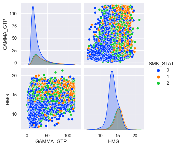
원칙적으로 ANOVA 분석을 통해서 SMK_STAT이 (0,2)/(1,2)인 그룹으로 각각 묶어서 p-value를 비교해야 하지만 Scatter plot을 통해 시각적으로 확인이 가능하므로 생략하자. 2는 1에 가까우므로 1으로 취급한다.

In principle, through ANOVA analysis, the p-value should be compared by grouping SMK_STAT into groups with (0,2)/(1,2), but it can be visually confirmed through the Scatter plot, so let's skip it. Since 2 is close to 1, treat it as 1.

Training and Testing

Split to Trainset and Testset

Trainset에서 8:2의 비율로 학습집단과 검증집단으로 분리한다.

In Trainset, it is divided into a training group and a testing group at a ratio of 8:2.

# x는 SMK_STAT column을 제외한 모든 column
x = smoke.loc[:,smoke.columns != 'SMK_STAT'].values

# y는 SMK_STAT column
y = smoke.loc[:,smoke.columns == 'SMK_STAT'].values

# Split dataset into train and test subsets
x_train2, x_test2, y_train, y_test = train_test_split(x,y,test_size = 0.20)

정규화(standardization)

# Standardize features by removing mean and scaling to unit variance
ss_train = StandardScaler()
x_train = ss_train.fit_transform(x_train2)

ss_test = StandardScaler()
x_test = ss_test.fit_transform(x_test2)

다양한 머신러닝 모델의 성능 검증(Verifying the performance of various machine learning models)

머신러닝 모델의 성능 검증을 통해 가장 우수한 모델을 채택한다. 사용 모델은 Logistic regression, Support vector machine, Decision Trees, Random forest, Naive bayes, K- Nearest Neighbors이다.

We adopt the best model through performance verification of machine learning models. Models used are Logic regression, Support vector machine, Decision Trees, Random Forest, Naive Bayes, and K-Nearest Neighbors.

<모델 구성(Model Configuration)>

# Try different models
models = {}

# Logistic Regression
from sklearn.linear_model import LogisticRegression
models['Logistic Regression'] = LogisticRegression()

# Support Vector Machines
from sklearn.svm import LinearSVC
models['Support Vector Machines'] = LinearSVC()

# Decision Trees
from sklearn.tree import DecisionTreeClassifier
models['Decision Trees'] = DecisionTreeClassifier()

# Random Forest
from sklearn.ensemble import RandomForestClassifier
models['Random Forest'] = RandomForestClassifier()

# Naive Bayes
from sklearn.naive_bayes import GaussianNB
models['Naive Bayes'] = GaussianNB()

# K-Nearest Neighbors
from sklearn.neighbors import KNeighborsClassifier
models['K-Nearest Neighbor'] = KNeighborsClassifier()

<성능 평가(Performance Assessment)>

from sklearn.metrics import accuracy_score, precision_score, recall_score, f1_score
from sklearn.model_selection import GridSearchCV

accuracy, precision, recall, f1 = {}, {}, {}, {}

for key in models.keys():
    
    # Fit the classifier
    models[key].fit(x_train, np.ravel(y_train))
    
    # Make predictions
    y_pred = models[key].predict(x_test)
    
    # Calculate metrics
    accuracy[key] = accuracy_score(y_pred, y_test)
    precision[key] = precision_score(y_pred, y_test)
    recall[key] = recall_score(y_pred, y_test)
    f1[key] = f1_score(y_pred, y_test)
    
df_model = pd.DataFrame(index=models.keys(), columns=['F1 Score', 'Accuracy', 'Precision', 'Recall'])
df_model['F1 Score'] = f1.values()
df_model['Accuracy'] = accuracy.values()
df_model['Precision'] = precision.values()
df_model['Recall'] = recall.values()

df_model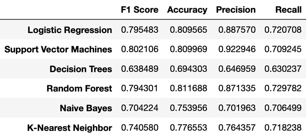

여러번의 시행을 거쳐본 결과 Support Vector Machine이 가장 성능이 우수해 이를 채택한다.

Parameter tunning

Hyperparameter tunning을 활용하여 support vector machine 에서의 최적 파라메터들을 구해내고 최종 score을 도출하자.

Let's use Hyperparameter tuning to find the optimal parameters in the support vector machine and derive the final score.

# x는 SMK_STAT column을 제외한 모든 column
x = smoke.loc[:,smoke.columns != 'SMK_STAT'].values

# y는 SMK_STAT column
y = smoke.loc[:,smoke.columns == 'SMK_STAT'].values

# Split dataset into train and test subsets
x_train2, x_test2, y_train, y_test = train_test_split(x,y,test_size = 0.20)


from sklearn.model_selection import GridSearchCV
from sklearn.svm import SVC

estimator = SVC() 

param_grid = {'kernel':['rbf'], 'C':[1,100,10,0.1,0.01,0.001]}
param_grid = [ 
{'kernel':['linear'], 'C':[1,100,10,0.1,0.01,0.001]}, #특정 하이퍼 파라메타 조합 피하기
{'kernel':['poly','rbf'], 'C':[1,100,10,0.1,0.01,0.001], 'gamma':['auto','scale',1000,100,10,1,0.1,0.01,0.001,0.0001]}]

grid = GridSearchCV(estimator, param_grid=param_grid) 
grid = GridSearchCV(estimator, param_grid=param_grid, cv=3, scoring='accuracy') #디폴트로 cv=3, 분류에서 디폴트로 scoring='accuracy'

grid.fit(x_train2, y_train)

print(grid.best_score_)
print(grid.best_params_)

사실 이 부분은 대회때는 하지 못하고 혼자 해보고 있는데 2시간 이상 걸리고 있는 상황이다. 튜닝이 마무리되는 시점을 정확히 몰라 마무리 되는 대로 결과치는 업데이트 시킬 예정이다.

글을 마무리 지으면서... (Conclusion)

나는 사람의 대략적인 건강상태를 통해서 흡연 유무를 구분하는 것이 쉽지 않을 것이라 예측했었지만 feature을 어떻게 잘 사용할지를 고민하는 과정에서 여러가지 시도를 해보며 accuracy 및 F1 score가 향상되는 것을 보며 많은 성취감을 느꼈다.

이 모델을 통해 우리 팀은 Field Camp에서 최우수상을 수상했고 교수님들께 피드백을 받으면서 내가 데이터엔지니어링을 공부한다면 무엇을 좀 더 신경써야 하는지를 배울 수 있었다.

추후 계획은 통계학에 대한 깊이있는 공부를 좀 더 해볼 생각이고 이를 기반으로 여러 머신러닝 모델이 어떤 특성의 변수에서 효과적으로 작동할 수 있을지를 판단하는 안목을 기르고자 한다.

At first I assumed that it would not be easy to distinguish smoker and non-smoker through a person's approximate health condition. I felt a lot of achievement when I saw the improvement of accuracy and F1 score while trying many things in the process of thinking about how to use feature well.

Through this model, our team won the best prize at Field Camp. Thanks to the feedback from the professors, I learned what to pay more attention to if I study data engineering.

The future plan is to study statistics in more depth, and based on this, I want to have an eye for determining which variables of characteristics several machine learning models can operate effectively.