해당 글은 제로베이스데이터스쿨 학습자료를 참고하여 작성되었습니다

TensorFlow 소개

• 머신러닝을 위한 오픈소스 플랫폼 - 딥러닝 프레임워크
• 구글이 주도적으로 개발 - 구글 코랩에는 기본 장착
• Keras라고 하는 고수준 API를 병합

Tensorflow의 의미

• Tensor : 벡터나 행렬
• Graph : 텐서가 흐르는 경로(혹은 공간)
• TensorFlow : 텐서가 Graph를 통해 흐른다

1.딥러닝의 기초 feat. Keras

• 신경망에서 아이디어를 얻어서 시작된 Neural Net

뉴런

• 구성요소 : 입력, 가중치, 활성화함수, 출력
• 가중치를 업데이트
• 처음에는 초기화를 통해 랜덤값을 넣고, 학습을 통해 가중치를 수렴시킴

레이어와 망(net)

• 뉴런이 모여서 layer를 구성하고, 망(net)이 됨

딥러닝

• 신경망이 깊어(많아)지면 깊은 신경망 Deep Learning이 됨

간단한 딥러닝의 목표

• 입력데이터(나이, 몸무게)로 출력데이터(혈중 지방) 얻기
• 선형회귀
• 뉴런 1개 사용하기

데이터 로딩

import numpy as np

raw_data = np.genfromtxt("../data/x09.txt", skip_header=36)

from mpl_toolkits.mplot3d import Axes3D
import matplotlib.pyplot as plt
%matplotlib inline

xs = np.array(raw_data[:,2], dtype=np.float32)
ys = np.array(raw_data[:,3], dtype=np.float32)
zs = np.array(raw_data[:,4], dtype=np.float32)

fig = plt.figure()
ax = fig.add_subplot(111, projection='3d')
ax.scatter(xs, ys, zs)
ax.set_xlabel("Weight")
ax.set_ylabel("Age")
ax.set_zlabel("Blood fat")
ax.view_init(15, 15)
plt.show()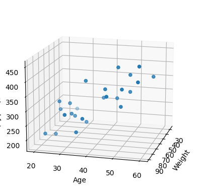

현재 목표

데이터 전처리

• 계산식 : $y = XW + b$
• x는 피쳐가 2개로 (row, 2)의 구조이다
• w는 벡터 계산으로 1개의 값을 얻어야하므로 (2, 1)의 구조를 갖는다
• b는 1개의 칼럼으로 상수를 갖으므로 (row, 1)의 구조이다
• y_data는 (25,)이므로 (25,1)로 변경해서 배열계산이 가능한 구조로 변경한다

x_data = np.array(raw_data[:, 2:4], dtype=np.float32)
y_data = np.array(raw_data[:, 4], dtype=np.float32)

y_data = y_data.reshape((25,1))

Sequential

• model의 layer를 순차적(sequential)으로 만든다
• 다른 모델도 많지만 사용할 때 알아보자

Dense

• 레이어의 출력=다음 입력일 때 완전히 연결된 fully connected 라고 함
• 이것을 시각적으로 "빽빽하게" 선들이 연결되므로 "Dense"라고 줄여서 씀
• Dense(출력, 입력, 활성화 함수)(아래에서 활성화 함수는 생략)

model.compile

• model을 만들 때 compile을 사용함
• loss는 "Mean Square Error"를 사용하고
• 오차를 최적화할 optimizer는 "Root Mean Square Propatation"를 사용한다
  • rmsprop는 기울기 강하의 속도를 증가시키는 알고리즘

import tensorflow as tf

model = tf.keras.models.Sequential([
    tf.keras.layers.Dense(1, input_shape=(2,)),
])

model.compile(optimizer="rmsprop", loss="mse")

model.summary()

• model의 요약내용을 보여줌
• 총 3개의 파라미터(weight 2개, bias 1개)를 찾아야함

model.summary()
-----------------------------------------------------------------
Model: "sequential_3"
_________________________________________________________________
 Layer (type)                Output Shape              Param #   
=================================================================
 dense_3 (Dense)             (None, 1)                 3         
                                                                 
=================================================================
Total params: 3
Trainable params: 3
Non-trainable params: 0
_________________________________________________________________

model.fit

• 모델을 학습시키는 명령어
• epochs: 반복횟수

hist = model.fit(x_data, y_data, epochs=5000)
-------------------------------------------------
Epoch 1/5000
1/1 [==============================] - 1s 546ms/step - loss: 83969.2109
Epoch 2/5000
1/1 [==============================] - 0s 6ms/step - loss: 83771.1562
...
Epoch 4999/5000
1/1 [==============================] - 0s 5ms/step - loss: 1979.2825
Epoch 5000/5000
1/1 [==============================] - 0s 5ms/step - loss: 1979.0133

loss 그래프 해석

• loss는 빠르게 감소하여 약 epoch=2400부터 수렴하기 시작함
• 이런 그래프가 좋은 결과

plt.plot(hist.history['loss'])
plt.title("model loss")
plt.xlabel("epochs")
plt.ylabel("loss")
plt.show()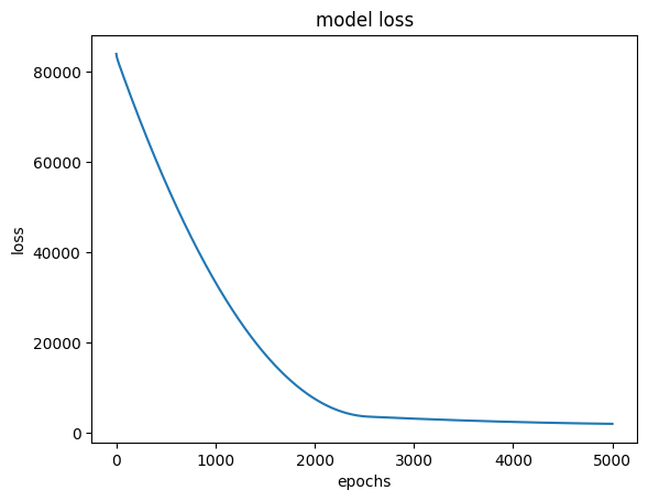

가중치와 bias 확인

W_, b_ = model.get_weights()
print("Weight is : \n", W_)
print("\nbias is : ", b_)
--------------------------------
Weight is : 
 [[1.734947 ]
 [4.7017527]]

bias is :  [4.966333]

test_data로 검증

• 임시로 검증데이터 제작

x = np.linspace(20, 100, 50).reshape(50, 1) # 몸무게
y = np.linspace(10, 70, 50).reshape(50, 1)  # 나이

X = np.concatenate((x,y), axis=1)           # 피쳐(몸무게+나이)
Z = np.matmul(X, W_) + b_           # 혈중 지방
fig = plt.figure(figsize=(12,12))
ax = fig.add_subplot(111, projection='3d')
ax.scatter(xs, ys, zs)
ax.scatter(x, y, Z)
ax.set_xlabel("Weight")
ax.set_ylabel("Age")
ax.set_zlabel("Blood fat")
ax.view_init(15, 15)
plt.show()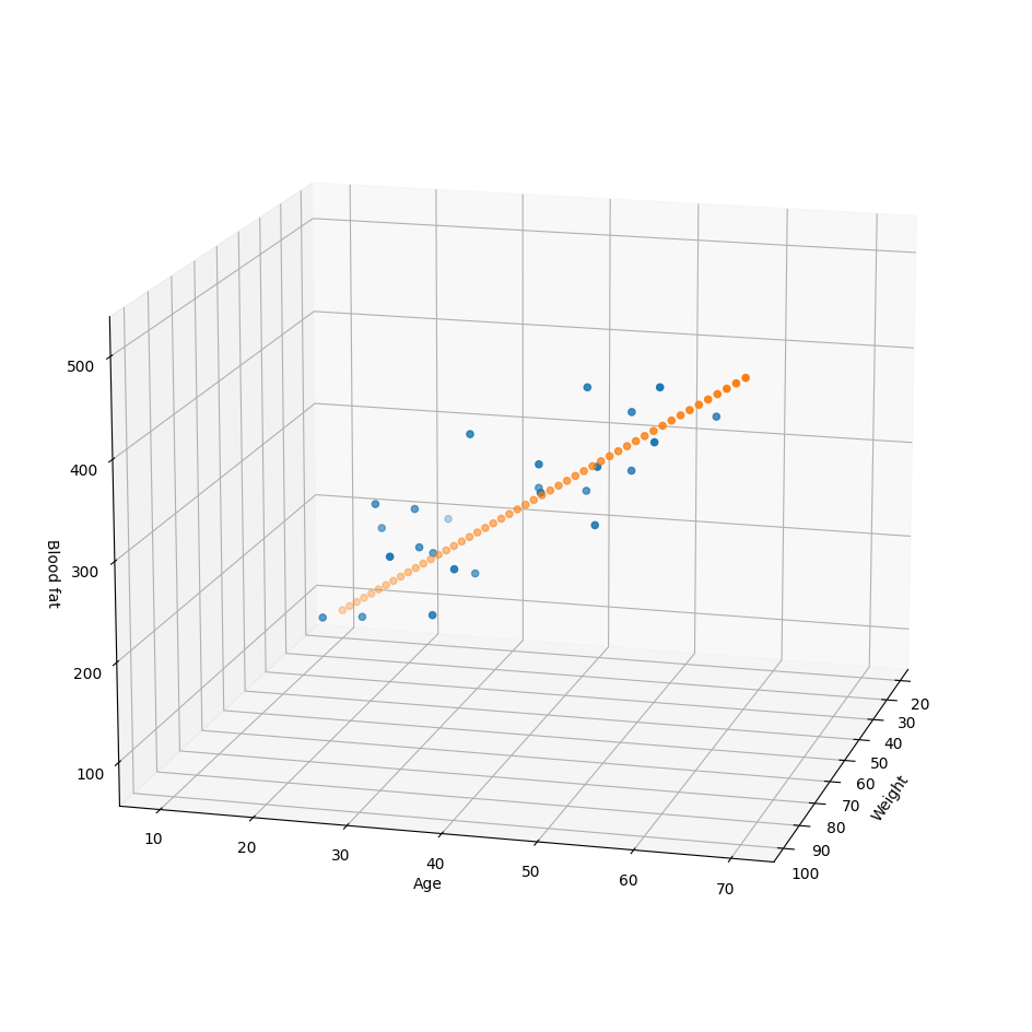

2. XOR Problem

import numpy as np

X = np.array([[0,0],
              [1,0],
              [0,1],
              [1,1]])
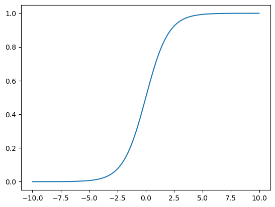
y = np.array([[0],[1],[1],[0]])

활성함수 sigmoid

• 모델이 복잡한 문제를 해결하기 위해서는 출력이 비선형이어야 한다

• layer의 결과가 비선형이되도록 "sigmoid"를 사용

• $s(z)=\frac{1}{1+e^{-z}}$

모델의 구조

model = tf.keras.Sequential([
    tf.keras.layers.Dense(2, activation="sigmoid", input_shape=(2,)),
    tf.keras.layers.Dense(1, activation="sigmoid"),
])

optimizers.SGD

• Stochastic Gradient Descent(확률적경사하강법)
• 각 반복에서 무작위로 선택된 데이터 하위 집합의 기울기를 사용하여 매개변수를 업데이트
• 이러한 무작위성은 노이즈를 도입하여 모델이 지역 최소값에서 빠르게 탈출할 수 있게 해줌
• 대용량 데이터셋에서 효율적
• Adam, RMSEProp의 변형으로 사용됨

model.compile(optimizer=tf.keras.optimizers.SGD(learning_rate=0.1), loss="mse")
model.summary()
------------------------------------------------------------------
Model: "sequential_7"
_________________________________________________________________
 Layer (type)                Output Shape              Param #   
=================================================================
 dense_10 (Dense)            (None, 2)                 6         
                                                                 
 dense_11 (Dense)            (None, 1)                 3         
                                                                 
=================================================================
Total params: 9
Trainable params: 9
Non-trainable params: 0
_________________________________________________________________

epochs와 batch_size

• epochs : 전체 데이터를 학습하는 사이클을 의미하고 이를 몇번 할지 결정
• batch_size : 한번의 학습에 사용할 데이터 수
  • batch_size를 늘리면 속도가 빠르지만, 메모리가 많이 필요
  • batch_size를 감소시키면 학습이 덜 되므로 epochs의 증가가 필요
  • 이 둘을 최적화해서 사용하는 것이 중요

hist = model.fit(X, y, epochs=5000, batch_size=1)
-------------------------------------------------------------------
Epoch 1/5000
4/4 [==============================] - 0s 2ms/step - loss: 0.2654
Epoch 2/5000
4/4 [==============================] - 0s 2ms/step - loss: 0.2641
...
Epoch 4999/5000
4/4 [==============================] - 0s 3ms/step - loss: 0.0031
Epoch 5000/5000
4/4 [==============================] - 0s 2ms/step - loss: 0.0031

model.predict(X)
-----------------------------------------------------
1/1 [==============================] - 0s 134ms/step
array([[0.04780162],
       [0.94222987],
       [0.94238436],
       [0.05789753]], dtype=float32)

import matplotlib.pyplot as plt
%matplotlib inline

plt.plot(hist.history["loss"])
plt.title("model loss")
plt.xlabel("epochs"); plt.ylabel("loss")
plt.show()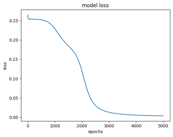

for w in model.weights:
    print("---")
    print(w)
--------------------------------------------------------------------
---
<tf.Variable 'dense_10/kernel:0' shape=(2, 2) dtype=float32, numpy=
array([[-5.702813 ,  3.8606172],
       [-5.7497272,  3.8687992]], dtype=float32)>
---
<tf.Variable 'dense_10/bias:0' shape=(2,) dtype=float32, numpy=array([ 2.0744014, -6.006867 ], dtype=float32)>
---
<tf.Variable 'dense_11/kernel:0' shape=(2, 1) dtype=float32, numpy=
array([[-7.6260552],
       [-7.7683024]], dtype=float32)>
---
<tf.Variable 'dense_11/bias:0' shape=(1,) dtype=float32, numpy=array([3.8022757], dtype=float32)>

분류 feat.iris

from sklearn.datasets import load_iris

iris = load_iris()

X = iris.data
y = iris.target

from sklearn.preprocessing import OneHotEncoder

ohe = OneHotEncoder(sparse=False, handle_unknown="ignore")
ohe.fit(y.reshape(len(y), 1))
ohe.categories_		# [array([0, 1, 2])]
y_ohe = ohe.transform(y.reshape(len(y), 1))
y_ohe
-------------------------------------------------
array([[1., 0., 0.],
       [1., 0., 0.],
       [1., 0., 0.],
...
       [0., 1., 0.],
       [0., 1., 0.],
       [0., 1., 0.],
...
       [0., 0., 1.],
       [0., 0., 1.],
       [0., 0., 1.]])

Net을 다음과 같이 구성한다

• 입력층 : 입력수 4개, 출력수 32개, 활성 relu
• 은닉층 : 활성 relu
• 출력층 : 출력수 3개, 활성 softmax

활성함수 softmax

• $softmax(x_i) = e^{x_i} / \sum_{j=1}^{n} e^{x_j}$
• 입력받은 값을 출력으로 0~1사이의 값으로 모두 정규화하며 출력 값들의 총합은 항상 1이 되는 특성을 가진 함수

활성함수 ReLU

• $f(x) = max(0, x)$
• +/-가 반복되는 신호에서 -흐름을 차단

활성함수

sigmoid의 한계

Vanishing Gradient problem

ReLU

• Rectified Linear Units
• 은닉층은 대부분 ReLU를 사용

softmax

• 카테고리들 중 확률이 가장 높은 대상을 정답으로 판단

Optimizer 정리

• optimizer는 loss를 최적화 하는 알고리즘

optimizers.Adam

• Adaptive Moment Estimation, Momentum + RMSProp

지수이동평균

m_t = beta1 * m_{t-1} + (1 - beta1) * g_t

v_t = beta2 * v_{t-1} + (1 - beta2) * g_t^2

편향보정

m_t_hat = m_t / (1 - beta1^t)

v_t_hat = v_t / (1 - beta2^t)

w_t = w_{t-1} - alpha * m_t_hat / (sqrt(v_t_hat) + epsilon)

모델구성

from sklearn.model_selection import train_test_split

X_train, X_test, y_train, y_test = train_test_split(X, y_ohe, test_size=0.2, random_state=13)
model = tf.keras.models.Sequential([
    tf.keras.layers.Dense(32, input_shape=(4, ), activation="relu"),
    tf.keras.layers.Dense(32, activation="relu"),
    tf.keras.layers.Dense(32, activation="relu"),
    tf.keras.layers.Dense(3, activation="softmax"),
])
# tf.keras.optimizers.Adam
# tf.keras.losses.categorical_crossentropy
# 많이 사용하는 optimizer와 loss는 문자로 입력해도 가능
model.compile(optimizer="adam", loss="categorical_crossentropy", metrics=["accuracy"])
model.summary()

hist = model.fit(X_train, y_train, epochs=100)
-------------------------------------------------------------------
Epoch 1/100
4/4 [==============================] - 1s 3ms/step - loss: 1.0497 - accuracy: 0.3500
Epoch 2/100
4/4 [==============================] - 0s 3ms/step - loss: 0.9938 - accuracy: 0.5000
...
Epoch 99/100
4/4 [==============================] - 0s 3ms/step - loss: 0.0612 - accuracy: 0.9833
Epoch 100/100
4/4 [==============================] - 0s 2ms/step - loss: 0.0661 - accuracy: 0.9667

model.evaluate(X_test, y_test, verbose=2)
-----------------------------------------------------------
1/1 - 0s - loss: 0.0776 - accuracy: 1.0000 - 29ms/epoch - 29ms/step
[0.07763615995645523, 1.0]

plt.plot(hist.history["loss"])
plt.plot(hist.history["accuracy"])
plt.legend(["loss", "accuracy"])
plt.xlabel("epochs"); plt.grid()
plt.show()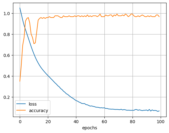

3. MNIST

• 입력층 : (784, 1000)
• 은닉층 : (1000, 1000), activation="relu"
• 출력층 : (1000, 10), activation="softmax"

import tensorflow as tf

mnist = tf.keras.datasets.mnist

(x_train, y_train),(x_test, y_test) = mnist.load_data()
x_train, x_test = x_train / 255.0, x_test / 255.0
x_train.shape, y_train.shape
-------------------------------------------------------------
((60000, 28, 28), (60000,))

Encoding

• 명목형 범주데이터는 OneHotEncoding 후 loss=categorical_crossentropy를 사용해야 하지만
• loss=sparse_categorical_crossentropy는 모델에서 위 2가지를 실행한다

Model

Modeling

model = tf.keras.models.Sequential([
    tf.keras.layers.Flatten(input_shape=(28, 28)),
    tf.keras.layers.Dense(1000, activation="relu"),
    tf.keras.layers.Dense(10, activation="softmax")
])

model.compile(optimizer="adam", loss=tf.losses.sparse_categorical_crossentropy,
              metrics=["accuracy"])
model.summary()
------------------------------------------------------------------------
Model: "sequential_15"
_________________________________________________________________
 Layer (type)                Output Shape              Param #   
=================================================================
 flatten_6 (Flatten)         (None, 784)               0         
                                                                 
 dense_28 (Dense)            (None, 1000)              785000    
                                                                 
 dense_29 (Dense)            (None, 10)                10010     
                                                                 
=================================================================
Total params: 795,010
Trainable params: 795,010
Non-trainable params: 0
_________________________________________________________________

Model Learning

import time

start_time = time.time()
hist = model.fit(x_train, y_train, validation_data=(x_test, y_test),
                 epochs=10, batch_size=100, verbose=1)
print("Fit time : ", time.time() - start_time)
---------------------------------------------------------------------
Epoch 1/10
600/600 [==============================] - 8s 13ms/step - loss: 0.1456 - accuracy: 0.9567 - val_loss: 0.0921 - val_accuracy: 0.9713
Epoch 2/10
600/600 [==============================] - 7s 12ms/step - loss: 0.0743 - accuracy: 0.9776 - val_loss: 0.0795 - val_accuracy: 0.9751
Epoch 3/10
600/600 [==============================] - 7s 12ms/step - loss: 0.0484 - accuracy: 0.9855 - val_loss: 0.0653 - val_accuracy: 0.9789
Epoch 4/10
600/600 [==============================] - 7s 12ms/step - loss: 0.0337 - accuracy: 0.9897 - val_loss: 0.0640 - val_accuracy: 0.9800
Epoch 5/10
600/600 [==============================] - 7s 12ms/step - loss: 0.0237 - accuracy: 0.9930 - val_loss: 0.0586 - val_accuracy: 0.9818
Epoch 6/10
600/600 [==============================] - 7s 12ms/step - loss: 0.0180 - accuracy: 0.9947 - val_loss: 0.0638 - val_accuracy: 0.9803
Epoch 7/10
600/600 [==============================] - 7s 12ms/step - loss: 0.0126 - accuracy: 0.9962 - val_loss: 0.0698 - val_accuracy: 0.9807
Epoch 8/10
600/600 [==============================] - 7s 12ms/step - loss: 0.0111 - accuracy: 0.9967 - val_loss: 0.0694 - val_accuracy: 0.9800
Epoch 9/10
600/600 [==============================] - 7s 12ms/step - loss: 0.0103 - accuracy: 0.9967 - val_loss: 0.0831 - val_accuracy: 0.9784
Epoch 10/10
600/600 [==============================] - 8s 13ms/step - loss: 0.0090 - accuracy: 0.9972 - val_loss: 0.0745 - val_accuracy: 0.9786
Fit time :  74.26960515975952

Model Learning History

plot_target = hist.history.keys()

plt.figure(figsize=(12, 8))
for each in plot_target:
    plt.plot(hist.history[each], label=each)
plt.legend(); plt.grid()
plt.show()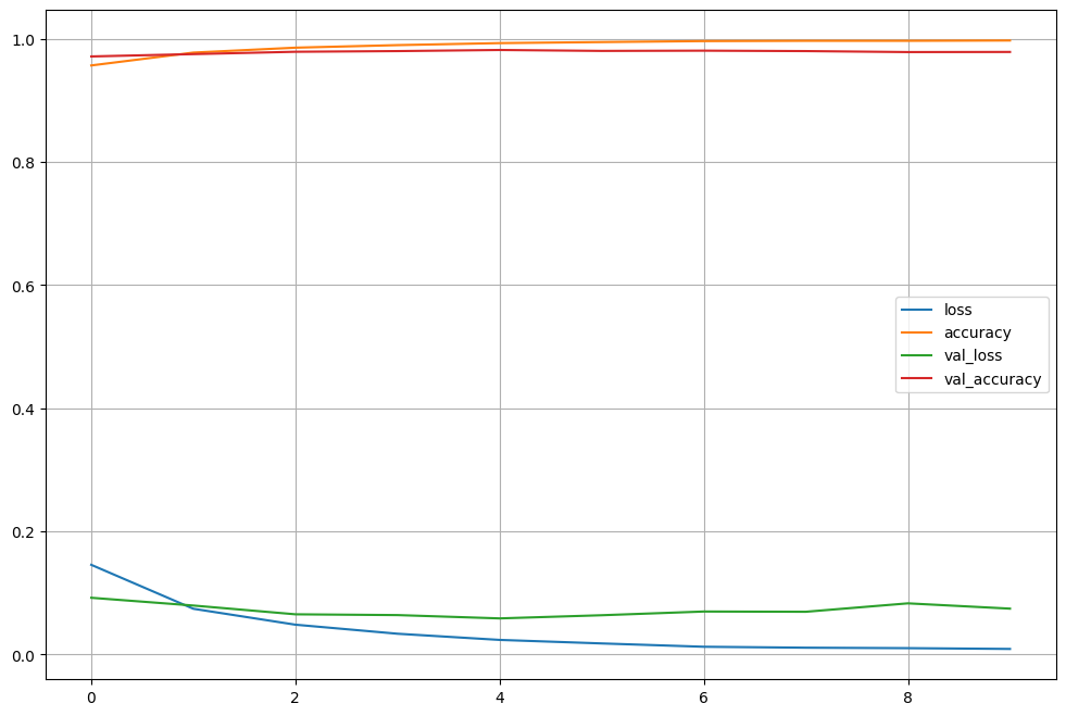

evaluation

score = model.evaluate(x_test, y_test)
print("Test loss :", score[0])
print("Train loss :", score[1])
---------------------------------------------------------
313/313 [==============================] - 1s 3ms/step - loss: 0.0745 - accuracy: 0.9786
Test loss : 0.07448840886354446
Train loss : 0.978600025177002

wrong_data_check

predicted_result = model.predict(x_test)
# np.argmax최대값의 인덱스 반환
predicted_labels = np.argmax(predicted_result, axis=1)
predicted_labels[:10]
y_test[:10]
-----------------------------------------------------
313/313 [==============================] - 1s 3ms/step
array([7, 2, 1, 0, 4, 1, 4, 9, 5, 9], dtype=int64)	# predict
array([7, 2, 1, 0, 4, 1, 4, 9, 5, 9], dtype=uint8)	# test_label

wrong_result = []

for n in range(0, len(y_test)):
    if predicted_labels[n] != y_test[n]:
        wrong_result.append(n)
        
len(wrong_result)
------------------------------------------------------
214	# 잘못된 데이터 갯수

import random

samples = random.choices(population=wrong_result, k=16)	# 잘못된 데이터의 인덱스 뽑기

plt.figure(figsize=(14,12))
for idx, n in enumerate(samples):
    plt.subplot(4, 4, idx+1)
    plt.imshow(x_test[n].reshape(28, 28), cmap="Greys")
    plt.title("Label : " + str(y_test[n]) + " Predict : " + str(predicted_labels[n]))
    plt.axis("off")
    
plt.show()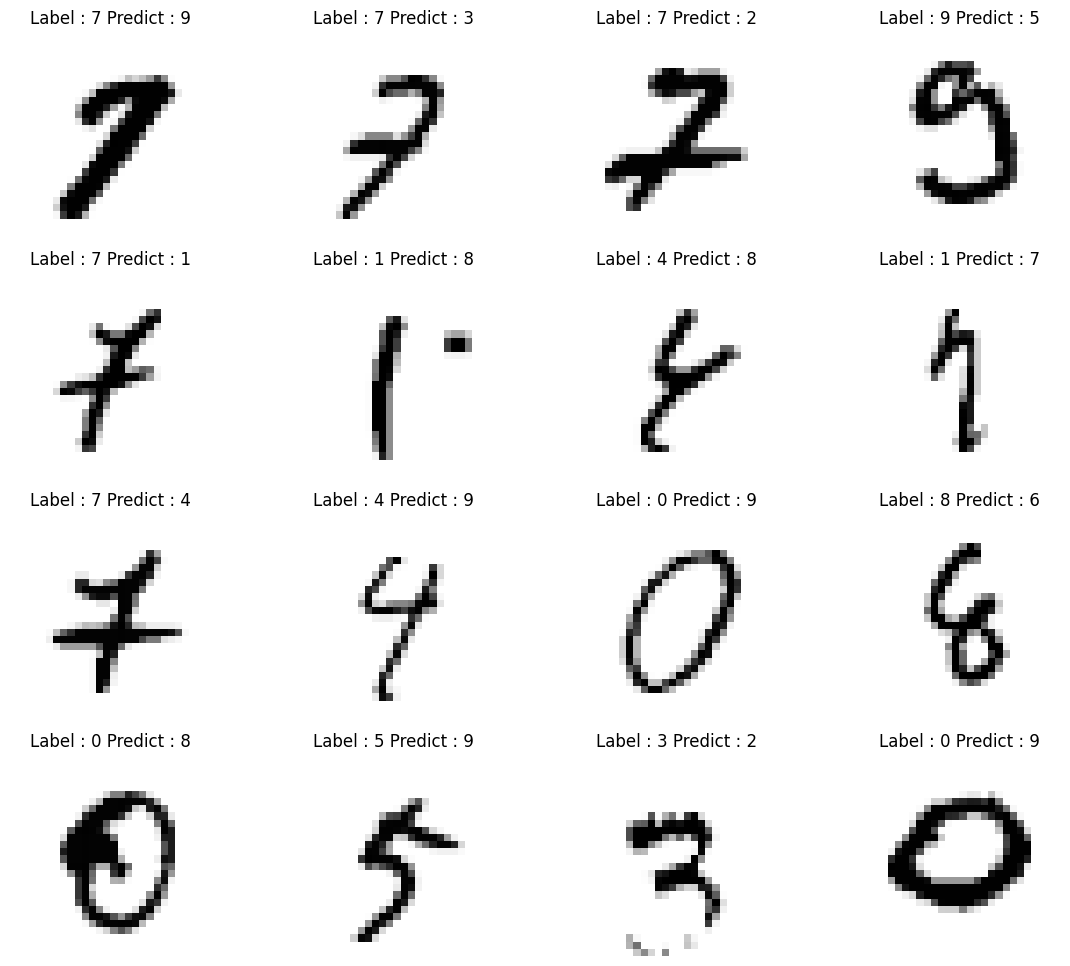

MNIST Fashion

DataLoad

import tensorflow as tf

fashion_mnist = tf.keras.datasets.fashion_mnist

(X_train, y_train), (X_test, y_test) = fashion_mnist.load_data()
X_train, X_test = X_train/255.0, X_test/255.0
smaples = random.choices(population=range(0, len(y_train)), k=16)

plt.figure(figsize=(14,12))

for idx, n in enumerate(samples):
    plt.subplot(4, 4, idx+1)
    plt.imshow(X_train[n].reshape(28, 28), cmap="Greys")
    plt.title("Label : " + str(y_train[n]))
    plt.axis("off")

Model

Modeling

model = tf.keras.models.Sequential([
    tf.keras.layers.Flatten(input_shape=(28, 28)),
    tf.keras.layers.Dense(1000, activation="relu"),
    tf.keras.layers.Dense(10, activation="softmax")
])

model.compile(optimizer="adam", loss=tf.losses.sparse_categorical_crossentropy,
              metrics=["accuracy"])
model.summary()
------------------------------------------------------------------------
Model: "sequential_18"
_________________________________________________________________
 Layer (type)                Output Shape              Param #   
=================================================================
 flatten_9 (Flatten)         (None, 784)               0         
                                                                 
 dense_34 (Dense)            (None, 1000)              785000    
                                                                 
 dense_35 (Dense)            (None, 10)                10010     
                                                                 
=================================================================
Total params: 795,010
Trainable params: 795,010
Non-trainable params: 0
_________________________________________________________________

Model Learning

import time

start_time = time.time()
hist = model.fit(X_train, y_train, validation_data=(x_test, y_test),
                 epochs=10, batch_size=100, verbose=1)
print("Fit time : ", time.time() - start_time)
-------------------------------------------------------------------------
Epoch 1/10
600/600 [==============================] - 9s 14ms/step - loss: 0.4836 - accuracy: 0.8285 - val_loss: 4.0778 - val_accuracy: 0.0973
Epoch 2/10
600/600 [==============================] - 8s 13ms/step - loss: 0.3616 - accuracy: 0.8690 - val_loss: 4.1924 - val_accuracy: 0.1019
Epoch 3/10
600/600 [==============================] - 7s 12ms/step - loss: 0.3228 - accuracy: 0.8826 - val_loss: 4.6794 - val_accuracy: 0.1027
Epoch 4/10
600/600 [==============================] - 8s 13ms/step - loss: 0.2958 - accuracy: 0.8921 - val_loss: 4.8663 - val_accuracy: 0.1036
Epoch 5/10
600/600 [==============================] - 8s 13ms/step - loss: 0.2793 - accuracy: 0.8960 - val_loss: 5.0290 - val_accuracy: 0.1026
Epoch 6/10
600/600 [==============================] - 8s 13ms/step - loss: 0.2652 - accuracy: 0.9011 - val_loss: 5.2187 - val_accuracy: 0.1066
Epoch 7/10
600/600 [==============================] - 7s 12ms/step - loss: 0.2505 - accuracy: 0.9061 - val_loss: 5.7567 - val_accuracy: 0.1018
Epoch 8/10
600/600 [==============================] - 7s 12ms/step - loss: 0.2397 - accuracy: 0.9100 - val_loss: 5.7923 - val_accuracy: 0.1023
Epoch 9/10
600/600 [==============================] - 8s 13ms/step - loss: 0.2295 - accuracy: 0.9133 - val_loss: 6.3656 - val_accuracy: 0.1014
Epoch 10/10
600/600 [==============================] - 7s 12ms/step - loss: 0.2204 - accuracy: 0.9181 - val_loss: 6.6526 - val_accuracy: 0.1029
Fit time :  76.89272260665894

Model Learning History

plot_target = hist.history.keys()

plt.figure(figsize=(12, 8))
for each in plot_target:
    plt.plot(hist.history[each], label=each)
plt.legend(); plt.grid()
plt.show()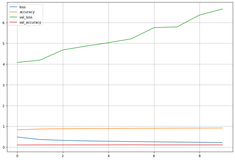

score = model.evaluate(X_test, y_test)
print("Test loss :", score[0])
print("Train loss :", score[1])
-----------------------------------------------------------------------------------------
313/313 [==============================] - 1s 3ms/step - loss: 0.3196 - accuracy: 0.8880
Test loss : 0.3196251392364502
Train loss : 0.8880000114440918

wrong_data_check

predicted_result = model.predict(X_test)
# np.argmax최대값의 인덱스 반환
predicted_labels = np.argmax(predicted_result, axis=1)
predicted_labels[:10]
y_test[:10]
---------------------------------------------------------------
array([9, 2, 1, 1, 6, 1, 4, 6, 5, 7], dtype=int64)	# predict
array([9, 2, 1, 1, 6, 1, 4, 6, 5, 7], dtype=uint8)	# test_label

wrong_result = []

for n in range(0, len(y_test)):
    if predicted_labels[n] != y_test[n]:
        wrong_result.append(n)
        
len(wrong_result)
------------------------------------------
1120

import random

samples = random.choices(population=wrong_result, k=16)

plt.figure(figsize=(14,12))
for idx, n in enumerate(samples):
    plt.subplot(4, 4, idx+1)
    plt.imshow(X_test[n].reshape(28, 28), cmap="Greys")
    plt.title("Label : " + str(y_test[n]) + " Predict : " + str(predicted_labels[n]))
    plt.axis("off")
    
plt.show()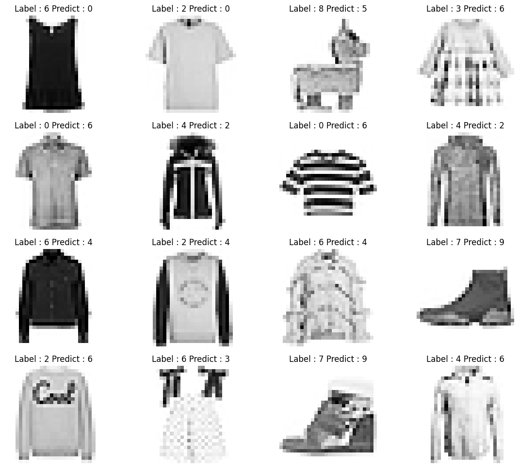

4. CNN

• Convolutional Neural Network
• 절차
  • 컨벌루션 + ReLU에서 변환
  • Maxpool에서 압축
  • 특징 검출된 압축된 사진을 얻음
  • Flatten()으로 펼쳐서 Dense에 입력
  • Dense를 구성하여 학습
  • 출력층에서 softmax로 결과도출

Dropout

파이썬 코드

DataLoad

import tensorflow as tf

mnist = tf.keras.datasets.mnist

(X_train, y_train),(X_test, y_test) = mnist.load_data()
X_train, X_test = X_train / 255.0, X_test / 255.0

X_train = X_train.reshape((60000, 28, 28, 1))
X_test = X_test.reshape((10000, 28, 28, 1))

Modeling

from tensorflow.keras import layers, models

model = models.Sequential([
    layers.Conv2D(32, kernel_size=(5,5), strides=(1,1), padding="same", activation="relu", input_shape=(28,28,1)),
    layers.MaxPooling2D(pool_size=(2,2), strides=(2,2)),
    layers.Conv2D(64, (2,2), activation="relu", padding="same"),
    layers.MaxPooling2D(pool_size=(2,2)),
    layers.Dropout(0.25),
    layers.Flatten(),
    layers.Dense(1000, activation="relu"),
    layers.Dense(10, activation="softmax")              
])

model.summary()
-----------------------------------------------------------------------------------------
Model: "sequential_19"
_________________________________________________________________
 Layer (type)                Output Shape              Param #   
=================================================================
 conv2d (Conv2D)             (None, 28, 28, 32)        832       
                                                                 
 max_pooling2d (MaxPooling2D  (None, 14, 14, 32)       0         
 )                                                               
                                                                 
 conv2d_1 (Conv2D)           (None, 14, 14, 64)        8256      
                                                                 
 max_pooling2d_1 (MaxPooling  (None, 7, 7, 64)         0         
 2D)                                                             
                                                                 
 dropout (Dropout)           (None, 7, 7, 64)          0         
                                                                 
 flatten_10 (Flatten)        (None, 3136)              0         
                                                                 
 dense_36 (Dense)            (None, 1000)              3137000   
                                                                 
 dense_37 (Dense)            (None, 10)                10010     
                                                                 
=================================================================
Total params: 3,156,098
Trainable params: 3,156,098
Non-trainable params: 0
_________________________________________________________________

Model Learning

import time

model.compile(optimizer="adam", loss="sparse_categorical_crossentropy", metrics=["accuracy"])

start_time = time.time()
hist = model.fit(X_train, y_train, epochs=5, verbose=1,
                 validation_data = (X_test,y_test))
print("Fit time : ", time.time() - start_time)
----------------------------------------------------------------------
Epoch 1/5
1875/1875 [==============================] - 90s 47ms/step - loss: 0.1150 - accuracy: 0.9639 - val_loss: 0.0370 - val_accuracy: 0.9887
Epoch 2/5
1875/1875 [==============================] - 87s 47ms/step - loss: 0.0453 - accuracy: 0.9857 - val_loss: 0.0329 - val_accuracy: 0.9887
Epoch 3/5
1875/1875 [==============================] - 101s 54ms/step - loss: 0.0328 - accuracy: 0.9892 - val_loss: 0.0225 - val_accuracy: 0.9931
Epoch 4/5
1875/1875 [==============================] - 133s 71ms/step - loss: 0.0247 - accuracy: 0.9919 - val_loss: 0.0237 - val_accuracy: 0.9931
Epoch 5/5
1875/1875 [==============================] - 119s 64ms/step - loss: 0.0210 - accuracy: 0.9934 - val_loss: 0.0376 - val_accuracy: 0.9897
Fit time :  530.8780899047852

Model Learning History

import matplotlib.pyplot as plt
%matplotlib inline

plot_target = hist.history.keys()
plt.figure(figsize=(12, 8))

for each in plot_target:
    plt.plot(hist.history[each], label=each)
    
plt.legend(); plt.grid()
plt.show()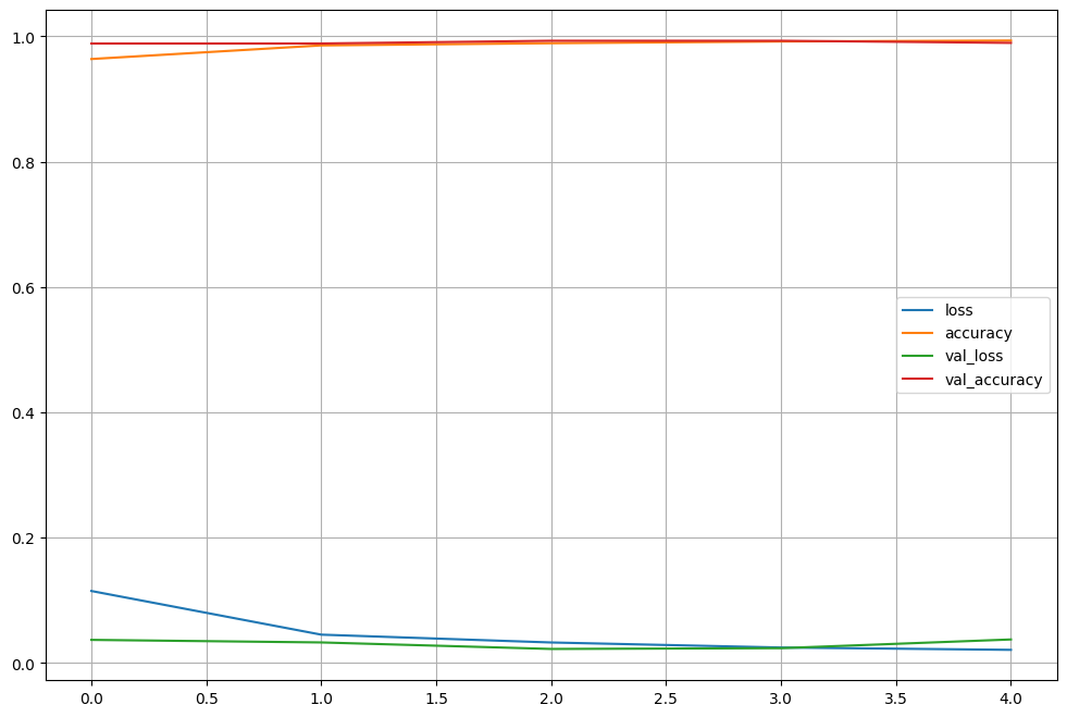

score = model.evaluate(X_test, y_test)
print("Test loss :", score[0])
print("Train loss :", score[1])
-----------------------------------------------------------------------
313/313 [==============================] - 4s 13ms/step - loss: 0.0376 - accuracy: 0.9897
Test loss : 0.037608176469802856
Train loss : 0.9897000193595886

wrong_data_check

predicted_result = model.predict(X_test)
# np.argmax최대값의 인덱스 반환
predicted_labels = np.argmax(predicted_result, axis=1)
predicted_labels[:10]
y_test[:10]
-------------------------------------------------------------
array([7, 2, 1, 0, 4, 1, 4, 9, 5, 9], dtype=int64)	# predict
array([7, 2, 1, 0, 4, 1, 4, 9, 5, 9], dtype=uint8)	# test_label

wrong_result = []

for n in range(0, len(y_test)):
    if predicted_labels[n] != y_test[n]:
        wrong_result.append(n)
        
len(wrong_result)
----------------------------------------------------------------
103

import random

samples = random.choices(population=wrong_result, k=16)

plt.figure(figsize=(14,12))
for idx, n in enumerate(samples):
    plt.subplot(4, 4, idx+1)
    plt.imshow(X_test[n].reshape(28, 28), cmap="Greys")
    plt.title("Label : " + str(y_test[n]) + " Predict : " + str(predicted_labels[n]))
    plt.axis("off")
    
plt.show()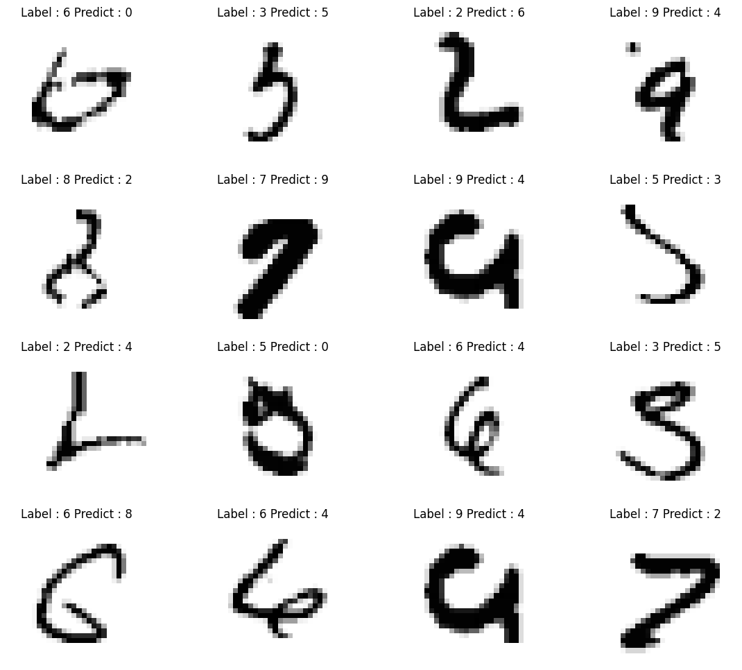

Model Save

import datetime

now_time = datetime.datetime.now().strftime("%Y%m%d-%H%M%S")
model.save(f"./checkpoint/MNIST_CNN_model_{now_time}.h5")