파이프라인

1. 파이프라인

📌 1. 파이프라인

• 여러 개의 데이터 처리 과정을 하나의 처리과정(pipneline, sequence)으로 만들어 데이터를 일괄 처리해주는 기능
• 더 짧은 코드로 가시성 있게 효율적으로 처리 가능
• 다양한 패키지에서 파이프라인 지원 중
  • 데이터 프레임 : Pandas, Polars
  • 머신러닝 : Scikit-Learn
  • 딥러닝 : Tensorflow, Pytorch

📌 2. Scikit-Learn의 파이프라인

• Pipeline 클래스를 통해 파이프라인 구현 가능
• 사용 목적
  • 편의성과 캡슐화 : 전체 데이터 처리 시퀀스에서 fit과 predict 한 번만 적용하면 됨
  • 통합된 하이퍼 파라미터 최적화 : grid search를 이용해 한 번에 하이퍼 파라미터 최적화 가능
  • 안전성 강화 : 교차검증(cross-validation) 시 랜덤성에 의한 데이터의 통계적 특성이 변경되는 것 방지

📌 3. 파이프라인 이용하기

• 라이브러리 불러오기

import pandas as pd
import numpy as np
from sklearn.feature_selection import SelectKBest, f_classif
from sklearn.preprocessing import StandardScaler
from sklearn.tree import DecisionTreeClassifier
from sklearn.datasets import load_iris

• 파이프라인 사용하지 않을 경우

#데이터셋 로드
x_data, y_data = load_iris(return_X_y=True)

#피쳐 셀렉팅
feat_sel = SelectKBest(f_classif, k =2)
X_selected = feat_sel.fit_transform(x_data, y_data)
print('Selected Feautures :', feat_sel.get_feature_names_out())

#표준화
scaler = StandardScaler()
scaler.fit(X_selected)
X_transformed = scaler.transform(X_selected)
print('Standard Scaled : \n', X_transformed[:5, :])

#모델학습
clf = DecisionTreeClassifier(max_depth = 3)
clf.fit(X_transformed, y_data)
print('Estimate : ', clf.predict(X_transformed)[:3])
print('Accuracy :', clf.score(X_transformed, y_data))

Selected Feautures : ['x2' 'x3']
Standard Scaled : 
 [[-1.34022653 -1.3154443 ]
 [-1.34022653 -1.3154443 ]
 [-1.39706395 -1.3154443 ]
 [-1.2833891  -1.3154443 ]
 [-1.34022653 -1.3154443 ]]
Estimate :  [0 0 0]
Accuracy : 0.9733333333333334

• 파이프라인 사용할 경우
  : 파이프라인은 (key, value)의 리스트 구성하여 만듦

from sklearn.pipeline import Pipeline

#데이터셋 로드
x_data, y_data = load_iris(return_X_y = True)

#pipeline 구축
pipeline = Pipeline([
    ('Feature Selection', SelectKBest(f_classif, k = 2)),
    ('Standardization', StandardScaler()),
    ('Decision Tree', DecisionTreeClassifier(max_depth = 3))
])
display(pipeline)

# 모형학습
pipeline.fit(x_data, y_data)

#예측과 성능 평가
print('Estimate : ', pipeline.predict(x_data)[:3])
print('Accuracy : ', pipeline.score(x_data, y_data))

Estimate :  [0 0 0]
Accuracy :  0.9733333333333334

• make_pipeline() 함수를 통해 파이프라인 생성 가능
  : 파이프라인 이름 자동으로 만들어 줌

from sklearn.pipeline import make_pipeline

pipeline_auto = make_pipeline(SelectKBest(f_classif, k = 2),
                               StandardScaler(),
                               DecisionTreeClassifier(max_depth = 3))
display(pipeline_auto)

2. 파이프라인의 결합

📌 1. 수치형 데이터 파이프라인 처리

• 라이브러리 불러오기

import seaborn as sns
import pandas as pd
from sklearn.pipeline import Pipeline
from sklearn.preprocessing import StandardScaler
from sklearn.impute import SimpleImputer

df = sns.load_dataset('diamonds')
print(df.info())
x_data = df.drop('price', axis = 1)
y_data = df['price']

numeric_col  = list(x_data.select_dtypes(exclude = 'category').columns)
category_col = list(x_data.select_dtypes(exclude = 'category').columns)
print(f'numeric_col  :  {numeric_col}')
print(f'category_col :  {category_col}')

<class 'pandas.core.frame.DataFrame'>
RangeIndex: 53940 entries, 0 to 53939
Data columns (total 10 columns):
 #   Column   Non-Null Count  Dtype   
---  ------   --------------  -----   
 0   carat    53940 non-null  float64 
 1   cut      53940 non-null  category
 2   color    53940 non-null  category
 3   clarity  53940 non-null  category
 4   depth    53940 non-null  float64 
 5   table    53940 non-null  float64 
 6   price    53940 non-null  int64   
 7   x        53940 non-null  float64 
 8   y        53940 non-null  float64 
 9   z        53940 non-null  float64 
dtypes: category(3), float64(6), int64(1)
memory usage: 3.0 MB
None
numeric_col  :  ['carat', 'depth', 'table', 'x', 'y', 'z']
category_col :  ['carat', 'depth', 'table', 'x', 'y', 'z']

• 파이프라인 만들기

numeric_pipl = Pipeline(
    steps = [
        ('imputer', SimpleImputer(strategy = 'mean')),
        ('scaler' , StandardScaler())
    ])
display(numeric_pipl)

#파이프라인 학습
numerical_data_piped = numeric_pipl.fit_transform(x_data[numeric_col])
pd.DataFrame(numerical_data_piped, columns = numeric_col).head()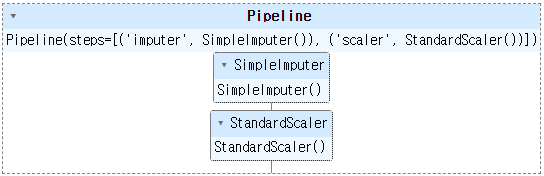

	carat		depth		table		x			y			z
0	-1.198168	-0.174092	-1.099672	-1.587837	-1.536196	-1.571129
1	-1.240361	-1.360738	1.585529	-1.641325	-1.658774	-1.741175
2	-1.198168	-3.385019	3.375663	-1.498691	-1.457395	-1.741175
3	-1.071587	0.454133	0.242928	-1.364971	-1.317305	-1.287720
4	-1.029394	1.082358	0.242928	-1.240167	-1.212238	-1.117674

📌 2. 범주형 데이터 파이프라인 처리

• 라이브러리 불러오기

from sklearn.impute import SimpleImputer
from sklearn.preprocessing import OneHotEncoder

• 파이프라인 만들기

categ_pipl = Pipeline(
    steps = [
        ('Imputer', SimpleImputer(strategy = 'constant')),
        ('onehot' , OneHotEncoder(sparse_output = False))
    ])
display(categ_pipl)

#파이프라인 학습
category_data_piped = categ_pipl.fit_transform(x_data[category_col])
#onehotencoder의 컬럼명 확인
category_colnames = categ_pipl[1].get_feature_names_out(category_col)
#파이프라인 이후 데이터(array -> dataframe)
pd.DataFrame(category_data_piped, columns = category_colnames).head()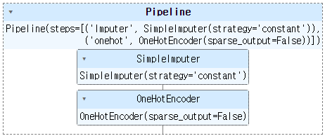

📌 3. 수치형 + 범주형 데이터 파이프라인 처리

• ColumnTransformer 클래스를 사용해 수치형과 범주형 데이터 파이프라인 결합 가능
• 필요한 라이브러리 불러오기

from sklearn.compose import ColumnTransformer
from sklearn.linear_model import LinearRegression
from sklearn.pipeline import make_pipeline

• 파이프라인 결합

preprocessor = ColumnTransformer(
    transformers = [
        ('numeric' , numeric_pipl, numeric_col),
        ('category', categ_pipl, category_col)
    ])

pipeln = make_pipeline(preprocessor, LinearRegression())
display(pipeln)
pipeln.fit(x_data, y_data)

print('Estimate : ', pipeln.predict(x_data))
print('Accuracy : ', pipeln.score(x_data, y_data))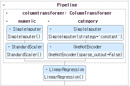

Estimate :  [ 737.67578125  451.25585938   56.00585938 ... 2429.54882812 3297.50585938
 3108.93359375]
Accuracy :  0.8938158297402341

📌 4. ColumnTransformer

: 컬럼 기준으로 데이터 복합하여 처리해주는 함수

• 라이브러리 불러오기

from sklearn.compose import ColumnTransformer
from sklearn.impute import SimpleImputer
import pandas as pd
import numpy as np

• ColumnTransformer 사용하기
  : SimpleImputer을 사용해 height의 null 값들은 평균으로 출력하고 나머지 column은 통과

data_df = pd.DataFrame({
    'height' : [165, np.nan, 182],
    'weight' : [70,  62, np.nan],
    'age'    : [np.nan, 18, 15]
})

# SimpleImputer을 사용해 height의 null 값들은 평균으로 출력하고 나머지 column은 통과
col_transform = ColumnTransformer([
    ('Impute_mean', SimpleImputer(strategy = 'mean'), ['height'])],
      remainder = 'passthrough')

display(col_transform)
print(data_df)
print(col_transform.fit_transform(data_df))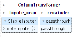

   height  weight   age
0   165.0    70.0   NaN
1     NaN    62.0  18.0
2   182.0     NaN  15.0
[[165.   70.    nan]
 [173.5  62.   18. ]
 [182.    nan  15. ]]

• ColumnTransformer 사용하기
  : SimpleImputer을 사용해 mean과 median값을 null에 넣고 나머지 column에 대한 값은 상수로 -1값을 넣어줌

col_transform2 = ColumnTransformer([
    ('Impute_mean'  , SimpleImputer(strategy = 'mean'), ['height']),
    ('Impute_median', SimpleImputer(strategy = 'median'), ['weight'])],
      remainder = SimpleImputer(strategy = 'constant', fill_value = 1))

display(col_transform2)
print(data_df)
print(col_transform2.fit_transform(data_df))

   height  weight   age
0   165.0    70.0   NaN
1     NaN    62.0  18.0
2   182.0     NaN  15.0
[[165.   70.    1. ]
 [173.5  62.   18. ]
 [182.   66.   15. ]]