
피쳐 엔지니어링
1. 피쳐 엔지니어링(Feature Engineering)
📌 1. 피쳐(Feature)
- 데이터 모델(특히 인공지능)에서 예측을 수행하는 데 사용되는 입력변수
- 피쳐의 유형
- 속성에 따라
- 범주형(categorical) : 범주나 순위가 있는 변수
- 수치형(numerical) : 수치로 표현되는 변수
- 범주형(categorical) : 범주나 순위가 있는 변수
- 인과관계에 따라
- 독립변수(independent variable) : 다른 변수에 영향을 받지 않고 종속변수에 영향을 주는 변수
- 종속변수(dependent variable) : 독립 변수로부터 영향을 받는 변수
- 독립변수(independent variable) : 다른 변수에 영향을 받지 않고 종속변수에 영향을 주는 변수
- 머신 러닝에서
- 입력(input) : 변수(feature),속성(attribute), 예측변수(predictor), 차원(Dimension), 관측치(Observation), 독립변수(independent variable)
- 출력(output) : 라벨(label), 클래스(class), 목표값(target), 반응(response), 종속변수(dependent variable)
- 입력(input) : 변수(feature),속성(attribute), 예측변수(predictor), 차원(Dimension), 관측치(Observation), 독립변수(independent variable)
- 속성에 따라
📌 2. 피쳐 엔지니어링(Feature Engineering)
: 머신 러닝 알고리즘의 성능을 향상시키기 위해 데이터에 대한 도메인 지식을 활용하여 변수를 조합하거나 새로운 변수 만드는 과정
-
피쳐 추출(feature extraction)
: 피쳐들 간 내재한 특성이나 관계 분석해 이들을 잘 표현할 수 있는 새로운 선형/비선형 결합변수 만들어 데이터 줄이는 방법
: 고차원 피쳐 공간을 저차원 공간으로 투영
: PCA(주성분 분석), LDA(선형 판별 분석) 등 -
피쳐 선택(feature selection)
: 피쳐 중 타겟에 가장 관련성이 높은 피쳐만을 선정해 피쳐 수 줄이는 과정
: 모델 단순화, train 시간 축소, 차원의 저주 방지, 과적합(Overfitting) 문제를 줄여 일반화해주는 장점 존재
: filter, wrapper, embedded method
2. 피쳐 추출(Feature Extraction)
📌 1. 피쳐 추출(Feature Extraction) 방법
: 피쳐들 간 내재한 특성이나 관계 분석해 이들을 잘 표현할 수 있는 새로운 선형/비선형 결합변수 만들어 데이터 줄이는 방법
- 주성분 분석(PCA, Principal Componenet Analysis)
: 변수들 간 공분산 행렬, 상관행렬 사용
: 고차원 공간의 표본들을 선형 연관성이 없는 저차원 공간으로 변환
: 행, 열의 수가 같은 정방행렬에서만 사용 - 선형판별분석(LDA, Linear Discriminant Analysis)
: 데이터의 target값 클래스끼리 최대한 분리 가능한 축 찾기
: 특정 공간상에서 클래스 분리를 최대화하는 축을 찾기 위한 클래스 간 분산(between-class scatter)과 클래서 내부 분산(within-class scatter) 비율을 최대화하는 방식으로 차원 축소 - 특이값 분해(Singular Value Decomposition)
: M X N 차원의 행렬데이터에서 특이값 추출하고 이를 통해 주어진 데이터셋을 효과적으로 축약할 수 있는 기법 - 요인 분석(Factor Analysis)
: 데이터 안에 관찰할 수 있는 잠재 변수(Latent Variable)가 존재한다고 가정
: 모형을 세운 뒤 잠재 요인 도출하고 데이터 내부 구조 해석하는 기법 - 독립 성분 분석(Independent component Analysis)
: 다변량의 신호를 통계적으로 독립적인 하부성분으로 분리해 차원 축소
: 독립성부의 분포는 비정규 분포를 따르게 되는 차원 축소 방법 - 다차원 척도법(Multi-Dimensional Scaling)
: 개체들 간 유사성, 비유사성 측정해 2차원 or 3차원 공간성에 점으로 표현해 개체들 간 집단화를 시각적으로 표현하는 분석 기법
📌 2. 주성분 분석(PCA)
- 목표 : 변환 결과인 차원 축소 벡터가 원래의 벡터와 유사하게 되는 W값 찾기
- 원 데이터의 분산을 최대한 보존하면서 서로 직교하는 새 기저(축)을 찾아 고차원 공간의 표본을 선형 연관성이 없는 저차원 공간으로 변환하는 기법
- 차원 축소는 고유값이 높은 순으로 정렬해 높은 고유값을 가지는 고유벡터만으로 데이터 복원(주성분)
- 낮은 고유값을 가진다 : 해당 고유벡터로는 변화(scale)가 작다
- 절차
- 학습 데이터셋에서 분산이 최대인 축(axis)을 찾음
- 첫번째 축과 직교(orthogonal)하면서 분산이 최대힌 두번째 축을 찾음
- 첫번째 축과 두번째 축에 직교하고 분산을 최대한 보존하는 세번째 축을 찾음
- 1~3과 같은 방법으로 데이터셋의 차원(특성 수)만큼 축을 찾음

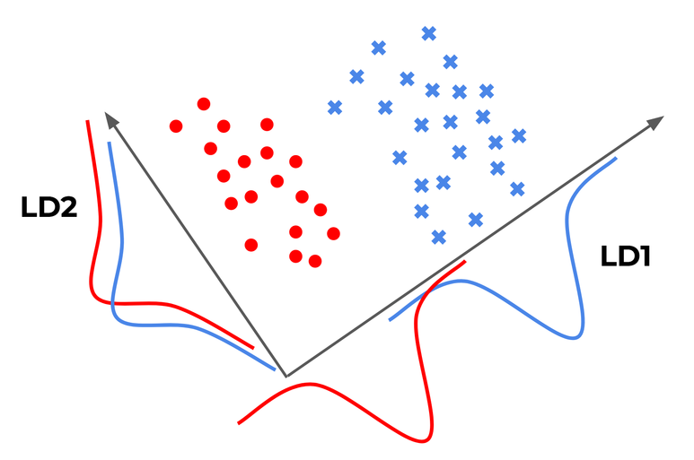
📌 3. 선형판별분석(LDA)
- 입력 데이터셋을 저차원 공간으로 투영해 차원 축소
- 데이터의 target 값 클래스끼리 최대한 분리할 수 있는 축 찾기 --> 지도학습
- PCA는 target 값을 사용하지 않기 때문에 비지도학습
- 투영 후 두 클래스 간 분산은 최대한 크게, 클래스 내부 분산은 최대한 작게 가져가는 방식
- [(클래스 간 분산) / (클래스 내부 분산)] 이 최대가 되도록 : 비율이 최대화되도록 차원 축소
📌 4. Scikit-learn으로 PCA/LDA 진행
- 필요한 라이브러리 불러오기
from sklearn import datasets
from sklearn.decomposition import PCA
from sklearn.discriminant_analysis import LinearDiscriminantAnalysis
iris = datasets.load_iris()
X = iris.data
y = iris.target
target_names = list(iris.target_names)
print(f"{X.shape = }, {y.shape = }")
print(f'{target_names = }')X.shape = (150, 4), y.shape = (150,)
target_names = ['setosa', 'versicolor', 'virginica']- PCA 수행하기
: 비지도 학습이기 때문에 y값 입력받지 않는다
# PCA 객체 생성하고 차원은 2차원으로 설정(현재 4차원)
pca = PCA(n_components = 2)

pca_fitted = pca.fit(X)

print(f'{pca_fitted.components_ =}')
print(f'{pca_fitted.explained_variance_ratio_ = }')

X_pca = pca_fitted.transform(X)   #주성분 벡터로 데이터 변환하기
print(f'{X_pca.shape = }')
pca_fitted.components_ =array([[ 0.36138659, -0.08452251, 0.85667061, 0.3582892 ],
[ 0.65658877, 0.73016143, -0.17337266, -0.07548102]])
pca_fitted.explained_variance_ratio_ = array([0.92461872, 0.05306648])
X_pca.shape = (150, 2)- LDA 수행하기
: 지도학습. y값(target)필요하다.
lda = LinearDiscriminantAnalysis(n_components = 2)

lda_fitted = lda.fit(X, y)

print(f'{lda_fitted.coef_ = }')
print(f'{lda_fitted.explained_variance_ratio_ = }')

X_lda = lda_fitted.transform(X)
print(f'{X_lda.shape = }')
lda_fitted.coef_ = array([[ 6.31475846, 12.13931718, -16.94642465, -20.77005459],
[ -1.53119919, -4.37604348, 4.69566531, 3.06258539],
[ -4.78355927, -7.7632737 , 12.25075935, 17.7074692 ]])
lda_fitted.explained_variance_ratio_ = array([0.9912126, 0.0087874])
X_lda.shape = (150, 2)- 시각화하기(plotting)
import matplotlib.pyplot as plt
#PCA plotting
plt.figure()
colors = ['navy', 'turquoise', 'darkorange']
lw = 2
for color, i, target_name in zip(colors, [0, 1, 2], target_names):
plt.scatter(
X_pca[y == i, 0], X_pca[y == i, 1], color = color, alpha = 0.8, lw = lw, label = target_name
)
plt.legend(loc = 'best', shadow = False, scatterpoints = 1)
plt.title("PCA of IRIS dataset")
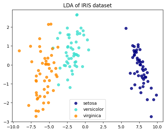
#LDA plotting
plt.figure()
for color, i, target_name in zip(colors, [0, 1, 2], target_names):
plt.scatter(
X_lda[y == i, 0], X_lda[y == i, 1], alpha = 0.8, color = color, label = target_name
)
plt.legend(loc = 'best', shadow = False, scatterpoints = 1)
plt.title("LDA of IRIS dataset")
plt.show()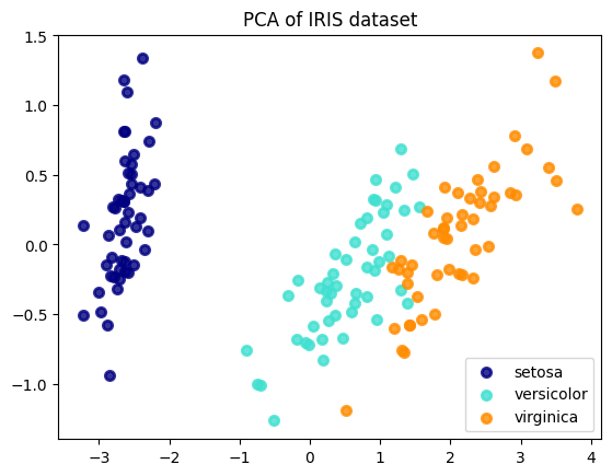
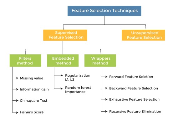
3. 피쳐 선택 기법
- 종속 변수 활용여부에 따라
- Supervised(지도) : 종속변수 활용해 선택
- Unsupervised(비지도) : 독립변수들만으로 선택
- 선택 메커니즘에 따라
- Filter : 통계적 방법으로 선택
- Wrapper : 모델 활용해 선택
- Embedded : 모델 훈련 과정에서 자동으로 선택
- Hybrid = Filter + Wrapper
📌 1. 필터 기법(Filter Method)
- 필요한 feature들만 선택해 feature-rank를 보여줌으로써 각 feature가 얼만큼의 영향력을 가지는지 보여주는 방식
- 통계적 방법으로 피쳐들 간 상관관계를 알아낸 뒤, 높은 상관계수(영향력)을 가지는 피쳐 사용
- 종류 : information gain, chi-square test, fisher score, correlation coefficient, variance threshold
- Scikit-learn 제공 피쳐 선택 기준
- f_classif : ANOVA F-value분류
- mutual_info_classif : 상호정보량(mutual information)분류
- chi2 : 카이제곱 분류
- f_regression : F-Value 회귀
- mutual_info_regression : 상호정보량 회귀
📋 F-value
: 두 모집단의 분산의 비율
: ANOVA, regression에서는 모형이 설명하는 분산/잔차의 분산 --> F-value가 크면 모형이 잘 설명하고 있다
📋 상호정보량
: 하나의 확률변수가 다른 하나의 확률변수에 대해 제공하는 정보의 양
: 두 확률변수가 공유하는 엔트로피 --> 상관관계가 강할수록 상호정보량 커짐, 독립이라면 상호정보량 0
- Scikit-learn 파이썬 코드 예시
from sklearn import datasets
from sklearn.feature_selection import VarianceThreshold

iris = datasets.load_iris()

X = iris.data
y = iris.target
X_names = iris.feature_names
y_names = iris.target_names

#분산이 0.2 이상인 피쳐들만 선택하도록 학습
sel = VarianceThreshold(threshold = 0.2).fit(X)
print(f"{sel.variances_ = }")

#분산이 0.2 이상인 피쳐들만 선택 적용
X_selected       = sel.transform(X)
X_selected_names = [X_names[i] for i in sel.get_support(indices = True)]

print(f"{X_selected_names = }")
print(f"{X_selected[:5] = }")
sel.variances_ = array([0.68112222, 0.18871289, 3.09550267, 0.57713289])
X_selected_names = ['sepal length (cm)', 'petal length (cm)', 'petal width (cm)']
X_selected[:5] = array([[5.1, 1.4, 0.2],
[4.9, 1.4, 0.2],
[4.7, 1.3, 0.2],
[4.6, 1.5, 0.2],
[5. , 1.4, 0.2]])from sklearn.feature_selection import SelectKBest
from sklearn.feature_selection import f_classif, f_regression, chi2
# K 개의 best feature 선택
####### f_classif
sel_cla = SelectKBest(f_classif, k = 2).fit(X, y)
print('f_classif : ')
print(f"{sel_cla.scores_ = }")
print(f"{sel_cla.pvalues_ = }")
print(f"{sel_cla.get_support() = }")
print("Selected features : ", [X_names[i] for i in sel_cla.get_support(indices=True)])
####### f_regression
sel_reg = SelectKBest(f_regression, k = 2).fit(X, y)
print("\nf_regression : ")
print(f"{sel_reg.scores_ = }")
print(f"{sel_reg.pvalues_ = }")
print(f"{sel_reg.get_support() = }")
print("Selected features : ", [X_names[i] for i in sel_reg.get_support(indices=True)])
####### chi2
sel_chi2 = SelectKBest(chi2, k = 2).fit(X, y)
print("\nchi2 : ")
print(f"{sel_chi2.scores_ = }")
print(f"{sel_chi2.pvalues_ = }")
print(f"{sel_chi2.get_support() = }")
print("Selected features : ", [X_names[i] for i in sel_chi2.get_support(indices=True)])f_classif :
sel_cla.scores_ = array([ 119.26450218, 49.16004009, 1180.16118225, 960.0071468 ])
sel_cla.pvalues_ = array([1.66966919e-31, 4.49201713e-17, 2.85677661e-91, 4.16944584e-85])
sel_cla.get_support() = array([False, False, True, True])
Selected features : ['petal length (cm)', 'petal width (cm)']
f_regression :
sel_reg.scores_ = array([ 233.8389959 , 32.93720748, 1341.93578461, 1592.82421036])
sel_reg.pvalues_ = array([2.89047835e-32, 5.20156326e-08, 4.20187315e-76, 4.15531102e-81])
sel_reg.get_support() = array([False, False, True, True])
Selected features : ['petal length (cm)', 'petal width (cm)']
chi2 :
sel_chi2.scores_ = array([ 10.81782088, 3.7107283 , 116.31261309, 67.0483602 ])
sel_chi2.pvalues_ = array([4.47651499e-03, 1.56395980e-01, 5.53397228e-26, 2.75824965e-15])
sel_chi2.get_support() = array([False, False, True, True])
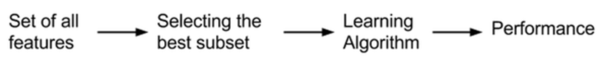
Selected features : ['petal length (cm)', 'petal width (cm)']📌 2. 래퍼 기법(Wrapper Method)
-
예측 정확도 측면에서 가장 좋은 성능을 보이는 featur subset(피쳐집합) 뽑아내기
-
기존 데이터에서 테스트를 진행할 hold-out set을 따로 두어야 한다.
-
최종적으로 best feature subset을 찾기 때문에 모델 성능 측면에서 매우 좋음
-
단 여러번 machine learning을 진행하기 때문에 시간과 비용이 많이 듦
-
변수선택 알고리즘
- 후진제거법(Backward Elimination)
: 모든 변수를 가지고 시작하며, 가장 덜 중요한 변수를 하나씩 제거하면서 성능 향상 - 전진선택법(Foward Selection)
: 변수가 없는 상태로 시작, 가장 중요한 변수를 하나씩 추가하며 성능의 향상이 없을때까지 진행 - 단계별 선택(Stepwise Selection)
: Foward + Backward 결합.
모든 변수를 가지고 시작하여 가장 도움이 되지 않는 변수를 삭제하거나 모델에서 빠져있는 변수 중 가장 중요한 변수 추가. 반대로 아무것도 없는 모델에서 시작할 수도 있다.
- 후진제거법(Backward Elimination)
-
종류
- RFE(Recursive Feature Elimination)
: SVM(support Vector Machine)을 사용해 재귀적으로 제거 - SFS(Sequential Feature Selection)
: 그리디 알고리즘(greedy algorithm)으로 빈 부분집합에서 특정 변수 하나씩 추가
- RFE(Recursive Feature Elimination)
-
Scikit-learn 파이썬 코드 예시
- RFE
from sklearn.datasets import load_iris
from sklearn.feature_selection import RFE, RFECV, SelectFromModel, SequentialFeatureSelector
from sklearn.svm import SVC, SVR

X, y = load_iris(return_X_y=True)

# 분류기 svc 객체 생성, 선형분류, 클래스 3개
svc = SVR(kernel='linear', C = 3)

# RFE 객체 생성, 2개의 피쳐 선택, 1개씩 제거
rfe = RFE(estimator=svc, n_features_to_select = 2, step = 1)
# RFE + CV(Cross Validation), 5개의 폴드, 1개씩 제거
rfe_cv = RFECV(estimator=svc, step = 1, cv = 5)

# RFE 적용
rfe.fit(X, y)
print('RFE Rank : ', rfe.ranking_)

X_selected = rfe.transform(X)
X_selected_names = [X_names[i] for i in rfe.get_support(indices=True)]

print(f"{X_selected_names = }")
print(f"{X_selected[:5] = }")

# RFECV 적용
rfe_cv.fit(X, y)
print('RFECV Rank : ', rfe_cv.ranking_)

X_selected = rfe_cv.transform(X)
X_selected_names = [X_names[i] for i in rfe_cv.get_support(indices=True)]

print(f"{X_selected_names = }")
print(f"{X_selected[:5] = }")
RFE Rank : [2 3 1 1]
X_selected_names = ['petal length (cm)', 'petal width (cm)']
X_selected[:5] = array([[1.4, 0.2],
[1.4, 0.2],
[1.3, 0.2],
[1.5, 0.2],
[1.4, 0.2]])
RFECV Rank : [1 2 1 1]
X_selected_names = ['sepal length (cm)', 'petal length (cm)', 'petal width (cm)']
X_selected[:5] = array([[5.1, 1.4, 0.2],
[4.9, 1.4, 0.2],
[4.7, 1.3, 0.2],
[4.6, 1.5, 0.2],
[5. , 1.4, 0.2]])- SFS
from sklearn.datasets import load_iris
from sklearn.feature_selection import SequentialFeatureSelector
from sklearn.neighbors import KNeighborsClassifier

X, y = load_iris(return_X_y=True)
knn  = KNeighborsClassifier(n_neighbors = 3)
sfs  = SequentialFeatureSelector(knn, n_features_to_select = 2, direction = 'backward')

# SFS 학습
sfs.fit(X, y)
print("SFS Selected : ", sfs.get_support())

X_selected = sfs.transform(X)
X_selected_names = [X_names[i] for i in sfs.get_support(indices = True)]

print(f"{X_selected_names = }")
print(f"{X_selected[:5] = }")
SFS Selected : [False False True True]
X_selected_names = ['petal length (cm)', 'petal width (cm)']
X_selected[:5] = array([[1.4, 0.2],
[1.4, 0.2],
[1.3, 0.2],
[1.5, 0.2],
[1.4, 0.2]])📌 3. 임베디드 기법(Embedded Method)
- Filter + Wrapper : 둘의 장점 결합
- 각각의 feature를 직접 학습하여 모델의 정확도에 기여하는 feature 선택
- 계수가 0이 아닌 feature가 선택되어 더 낮은 복잡성으로 모델을 훈련하고 학습 절차 최소화
- 방법
- LASSO : L1-norm을 통해 제약을 주는방법
- Ridge : L2-norm을 통해 제약을 주는 방법
- Elastic-net : 위 둘을 선형결합
- SelectFromModel : decision tree 기반 알고리즘에서 feature 선택 --> sklearn에 라이브러리 있다.
- Scikit-learn 파이썬 코드 예시
from sklearn.feature_selection import SelectFromModel
from sklearn import tree
from sklearn.datasets import load_iris

X, y = load_iris(return_X_y=True)

clf = tree.DecisionTreeClassifier()
sfm = SelectFromModel(estimator = clf)

sfm.set_output(transform = 'pandas')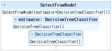
sfm.fit(X, y)
print('SFM threshold : ', sfm.threshold_)

X_selected = sfm.transform(X)
X_selected.columns = [X_names[i] for i in sfm.get_support(indices = True)]

X_selected.head()
SFM threshold : 0.25
petal width (cm)
0 0.2
1 0.2
2 0.2
3 0.2
4 0.2