google colab 을 이용하여 Ai 기초 다지기
# 한글 셋팅!!!!!!!!
!sudo apt-get install -y fonts-nanum
!sudo fc-cache -fv
!rm ~/.cache/matplotlib -rf
import numpy as np

test_list = ["one", 'two', 'three']

my_array = np.array(test_list)
print(my_array[2])
my_array.shape

len(test_list)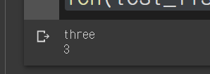
test_list = ["one", 'two', 'three']
for i in test_list:
  print(i)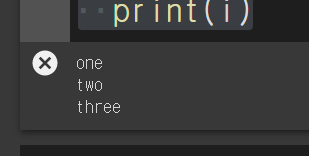
import numpy as np
np.set_printoptions(suppress =True, precision=4)

a=np.array([1,2,3,4,5,6,7])
print("a : ", a)
b=np.array([[1,2,3], [4,5,6],[7,8,9],[10,11,12]])
# 4 by 3 procession
print("b : ", b)

# 모양 (행렬처럼)
print(a.shape)
print(b.shape)

#  길이
print(len(a))
print(len(b))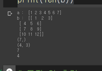
# 특정 열 출력
# : 은 '처음부터 끝까지' 를 의미한다. == '모든 행'
# 슬라이싱으로 모든 elements 에 접근해서 0 번째 배열의 값을 가져온다.
c=b[:,0]
print(c)

# 슬라이싱으로 모든 elements 에 접근해서 모든 배열의 값을 가져오는데, 2 번째 배열 전까지 가져온다.
d=b[:,:2]
print(d)

# 정수 12자리를 가지고 배열을 만들겠다.
test =np.array(range(12))
print(test)

# 이미 존재하는 배열을 shaping 하겠다.
m = test.reshape((3,4))
print(m)

# n = test.reshape((2.6))

# print(n)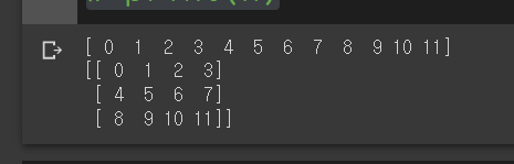
a =np.array(range(7))
print('원래 변수 ', a)

a_sum = np.sum(a)
print("합 :", a_sum)

a_mean = np.mean(a)
print("평균 :", a_mean)

a_max = np.max(a)
print("최댓값 :", a_max)

a_min = a.min()
print("최소값 :", a_min)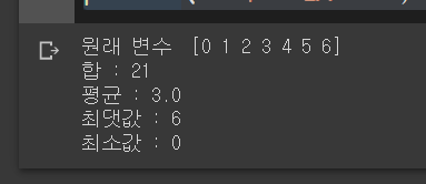
yt = np.array([1,1,1,1,1,1,1,0]);
yp = np.array([1,1,1,1,1,1,1,1]);
print(yt)
print(yp)
w =(yt == yp)
print(w)
print(w.sum())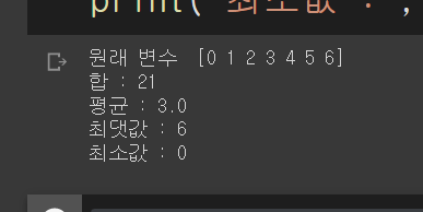
# slicing = :

list =[1,2,3,4,5,6,7,8,9,10,11,13,14,15]
print(list)
print()
print(list[2:6])
print(list[2])
print(list[:5])
print(list[:-1])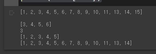
import matplotlib.pyplot as plt
r1000 = np.random.rand(1000)
plt.hist(r1000)
plt.grid()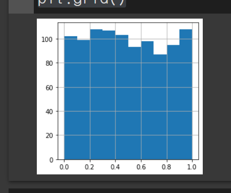
rn = np.random.normal(0, 1, 3)
print(rn)

rn1000 = np.random.normal(0,1,1000)
plt.hist(rn1000)
plt.grid()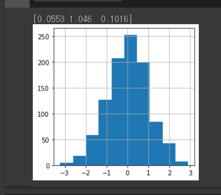
np.random.seed(0)
print(np.random.rand(3))
np.random.seed(0)
print(np.random.rand(3))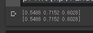
narray = np.array([1,3,5,7,9])
print('narray : ', narray)

darray = np.array([[1,3,5,7,9], [2, 4, 6, 8, 10]])
print('darray : ', darray)

d52 = darray.reshape(5,2)
print('d52 : ', d52)

d10 =darray.reshape(10,)
print('d10 : ', d10)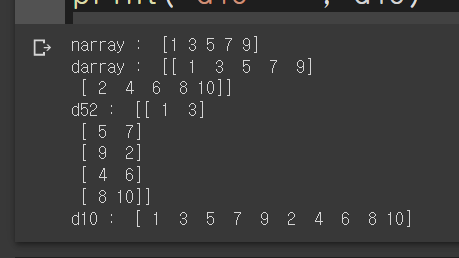
# !pip install -q xlrd
import pandas as pd
# df = pd.read_excel('test1.xlsx')
# df
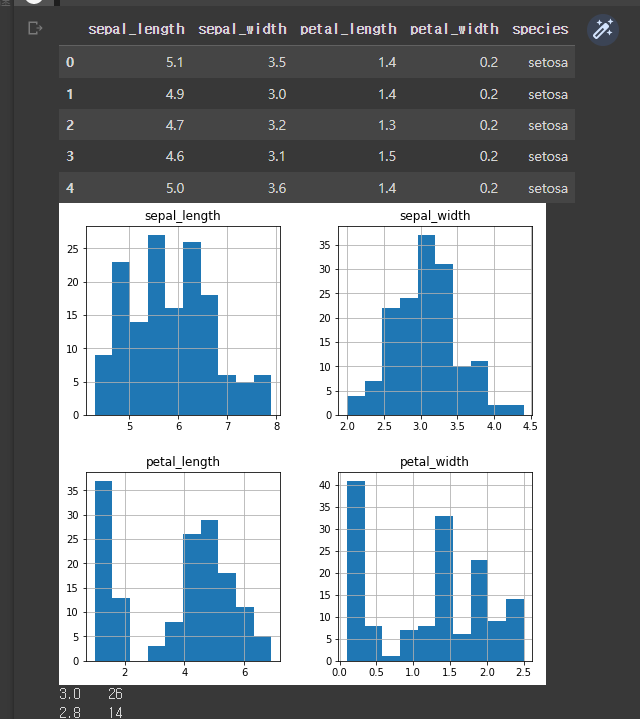
import seaborn as sns
df_iris = sns.load_dataset("iris")
display(df_iris.head())
xs = df_iris['sepal_length']
ys = df_iris['sepal_width']
plt.rcParams['figure.figsize'] = (6, 6)
plt.scatter(xs, ys)
plt.show()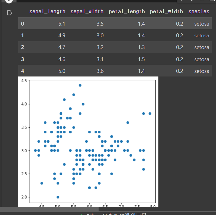
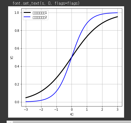
def sigmoid(x, a):
  return(1/(1 + np.exp(-a*x)))

xp = np.linspace(-3,3,61)

print(xp)

plt.rcParams['figure.figsize'] = (10,10)

plt.plot(xp, sigmoid(xp, 1.0))

plt.show()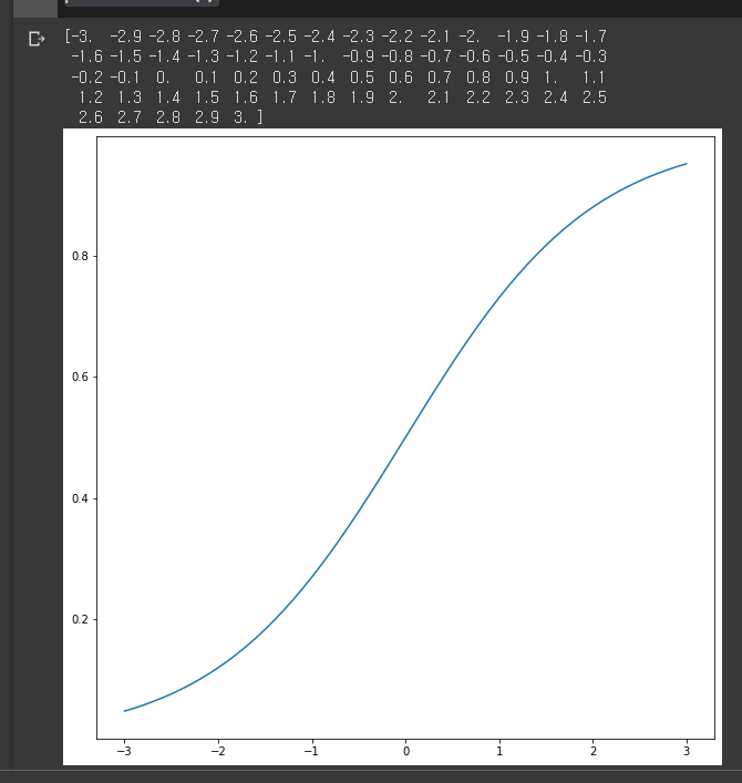
plt.rcParams['figure.figsize'] = (6,6)

# 두개의 다른 그래프 그리기
plt.plot(xp, sigmoid(xp, 1.0), label='시그모이드함수1', lw=3, c='k')

plt.plot(xp, sigmoid(xp, 2.0), label='시그모이드함수2', lw=2, c='b')

plt.grid()
plt.legend()
plt.xlabel('x축')
plt.ylabel('y축')

plt.show()
import seaborn as sns
df_iris = sns.load_dataset("iris")
display(df_iris.head())
xs = df_iris['sepal_length']
ys = df_iris['sepal_width']
###########################
plt.rcParams['figure.figsize'] = (8, 8)
# hist : 히스토 그램
df_iris.hist()
plt.show()
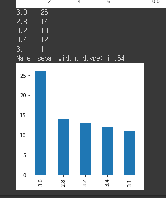
counts_ser = df_iris['sepal_width'].value_counts().iloc[:5]
print(counts_ser)
plt.rcParams['figure.figsize'] = (4, 4)
counts_ser.plot(kind='bar')
plt.show()