Regularization

L2 Regularization

The cost function of L2 regularization is as follows:

The formula is summation of cross-entropy cost and L2 regularization cost.

• sum up all elements in W and square it

def compute_cost_with_regularization(A3, Y, parameters, lambd):
    m = Y.shape[1]
    W1 = parameters["W1"]
    W2 = parameters["W2"]
    W3 = parameters["W3"]
    
    cross_entropy_cost = compute_cost(A3, Y) 

    L2_regularization_cost = lambd / m / 2 * (np.sum(np.square(W1)) + np.sum(np.square(W2)) + np.sum(np.square(W3)))
    
    cost = cross_entropy_cost + L2_regularization_cost
    
    return cost

Weight decay

The basic principle of L2 regularization is decaying weight by using $\lambda$. Decaying a weight means decreasing the value of $W$ by adding additional value in $dW$. As a result, more $\lambda$ you set, less $W$ you have.

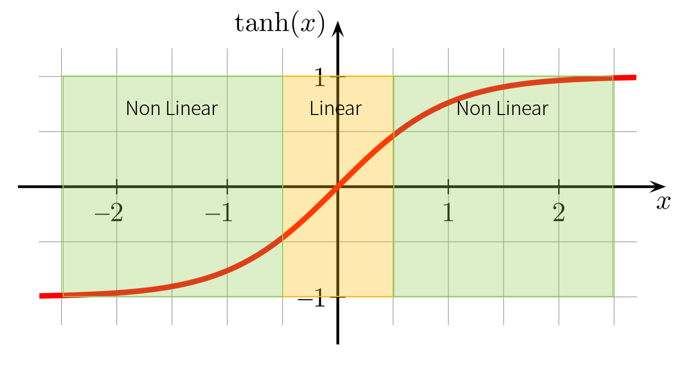
Normally, in activation function, the ranges which are close to zero is usually have linear form(line), but the ranges which are far from to zero is not linear. It means that if an argument of activation function is large, it is possible to make complicated decision which cause overfittin somtimes. By decreasing the value of $W$, it can prevent model from making very complicated decision.

Back propagation with regularization

The changes only concern additional L2 regularization part.

Add the term $\frac{\lambda}{m}W_i$ in each $dW_i$ terms.

def backward_propagation_with_regularization(X, Y, cache, lambd):
    m = X.shape[1]
    (Z1, A1, W1, b1, Z2, A2, W2, b2, Z3, A3, W3, b3) = cache
    
    dZ3 = A3 - Y
    dW3 = 1./m * np.dot(dZ3, A2.T) + lambd / m * W3
    db3 = 1. / m * np.sum(dZ3, axis=1, keepdims=True)
    
    dA2 = np.dot(W3.T, dZ3)
    dZ2 = np.multiply(dA2, np.int64(A2 > 0))
    dW2 = 1./m * np.dot(dZ2, A1.T) + lambd / m * W2

    db2 = 1. / m * np.sum(dZ2, axis=1, keepdims=True)
    
    dA1 = np.dot(W2.T, dZ2)
    dZ1 = np.multiply(dA1, np.int64(A1 > 0))
    
    dW1 = 1./m * np.dot(dZ1, X.T) + lambd / m * W1

    db1 = 1. / m * np.sum(dZ1, axis=1, keepdims=True)
    
    gradients = {"dZ3": dZ3, "dW3": dW3, "db3": db3,"dA2": dA2,
                 "dZ2": dZ2, "dW2": dW2, "db2": db2, "dA1": dA1, 
                 "dZ1": dZ1, "dW1": dW1, "db1": db1}
    
    return gradients

By using regularization, you can block overfitting data based on weight decay.

Dropout

The dropout is weakening neural network based on keep probability. According to probability, randomly, neglect some cells then it will shrink weight like L2 regularization.

Forward propagation with dropout

Main idea of implementing dropout in forward propagation is shutting down nerons based on keep_props. By multiplying matrix(elementwise multiplying) D with result of activation function, change elements in A into zero.
Last step is dividing the results with keep probability because it is necessary to scaling the value as already expected i.e. assuring the result of the cost will still have the same expected value as without dropoutp.

def forward_propagation_with_dropout(X, parameters, keep_prob = 0.5):
    # retrieve parameters
    W1 = parameters["W1"]
    b1 = parameters["b1"]
    W2 = parameters["W2"]
    b2 = parameters["b2"]
    W3 = parameters["W3"]
    b3 = parameters["b3"]
    
    # LINEAR -> RELU -> LINEAR -> RELU -> LINEAR -> SIGMOID
    Z1 = np.dot(W1, X) + b1
    A1 = relu(Z1)
    
    D1 = np.random.rand(A1.shape[0], A1.shape[1])
    D1 = (D1 < keep_prob).astype(int)
    A1 = A1 * D1
    A1 = A1 / keep_prob

    Z2 = np.dot(W2, A1) + b2
    A2 = relu(Z2)
    
    D2 = np.random.rand(A2.shape[0], A2.shape[1])
    D2 = (D2 < keep_prob).astype(int)
    A2 = A2 * D2
    A2 = A2 / keep_prob
   
    Z3 = np.dot(W3, A2) + b3
    A3 = sigmoid(Z3)
    
    cache = (Z1, D1, A1, W1, b1, Z2, D2, A2, W2, b2, Z3, A3, W3, b3)
    
    return A3, cache

You should keep D for back propagation process.

Backward propagation with dropout

First of all, use D1 and D2 in cache for shutting down exact same cells. Last step is dividing the results with keep_prop as same as forward propagation step.

def backward_propagation_with_dropout(X, Y, cache, keep_prob):
    m = X.shape[1]
    (Z1, D1, A1, W1, b1, Z2, D2, A2, W2, b2, Z3, A3, W3, b3) = cache
    
    dZ3 = A3 - Y
    dW3 = 1./m * np.dot(dZ3, A2.T)
    db3 = 1./m * np.sum(dZ3, axis=1, keepdims=True)
    dA2 = np.dot(W3.T, dZ3)
    
    dA2 = dA2 * D2
    dA2 = dA2 / keep_prob
    
    dZ2 = np.multiply(dA2, np.int64(A2 > 0))
    dW2 = 1./m * np.dot(dZ2, A1.T)
    db2 = 1./m * np.sum(dZ2, axis=1, keepdims=True)
    
    dA1 = np.dot(W2.T, dZ2)
    
    dA1 = dA1 * D1
    dA1 = dA1 / keep_prob
    
    dZ1 = np.multiply(dA1, np.int64(A1 > 0))
    dW1 = 1./m * np.dot(dZ1, X.T)
    db1 = 1./m * np.sum(dZ1, axis=1, keepdims=True)
    
    gradients = {"dZ3": dZ3, "dW3": dW3, "db3": db3,"dA2": dA2,
                 "dZ2": dZ2, "dW2": dW2, "db2": db2, "dA1": dA1, 
                 "dZ1": dZ1, "dW1": dW1, "db1": db1}
    
    return gradients

Reference

• deeplearning.ai