https://ocw.mit.edu/courses/18-06-linear-algebra-spring-2010/video_galleries/video-lectures/
먼저 vector projection에 대해서 알아보자.
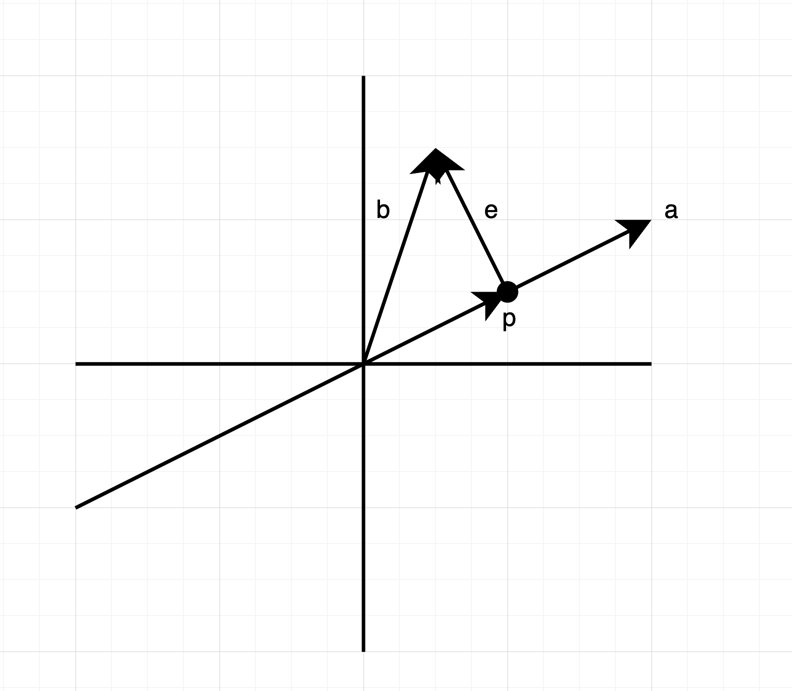
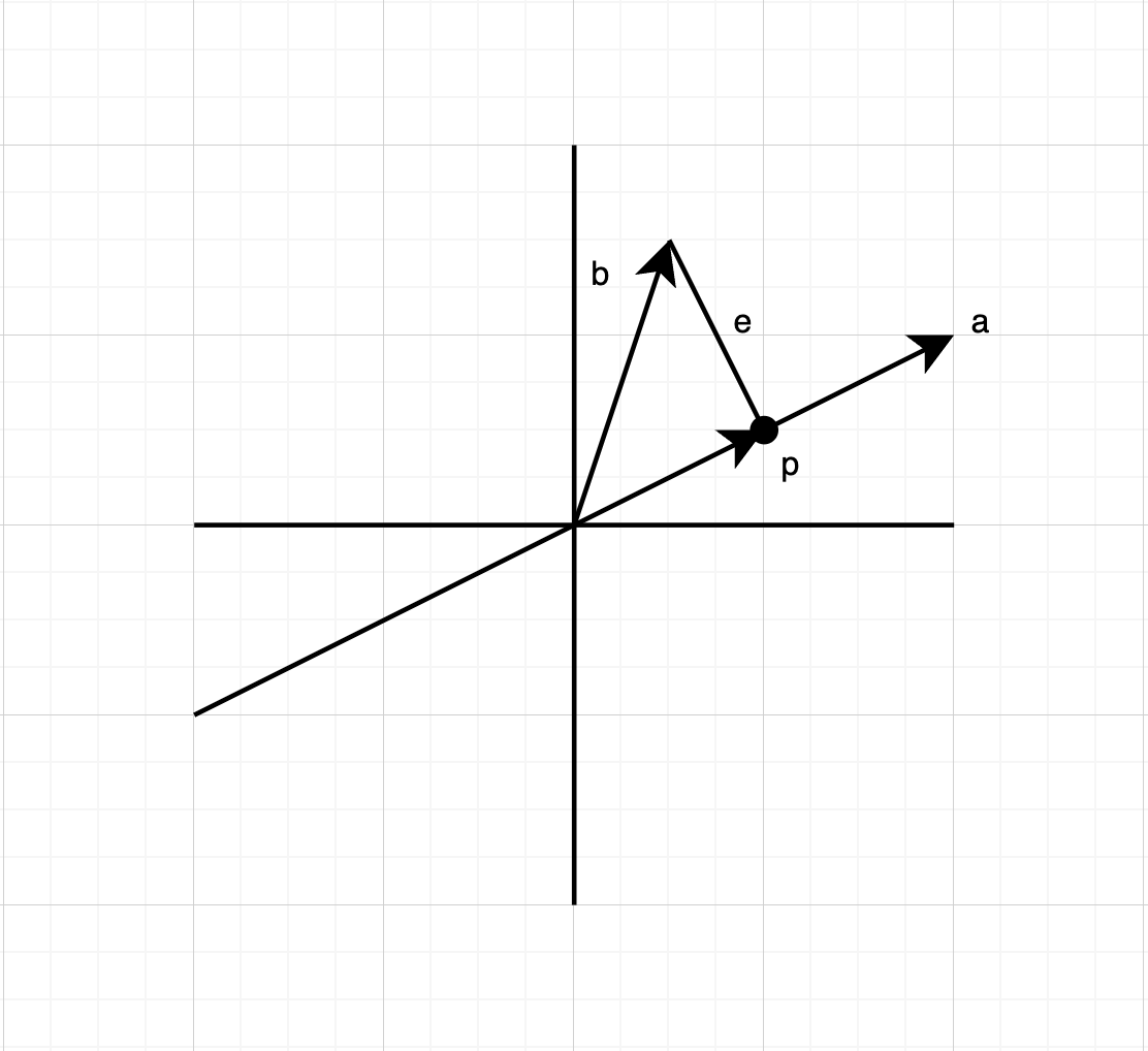
- 위 그래프처럼 벡터 a,b∈R1가 존재한다고 가정해보자. 두 벡터는 서로 다른 subspace에 존재한다.
- 그리고 벡터 b를 벡터 a 쪽으로 project한다. 이 projection을 p라고 하자.
- p는 a의 subspace에 존재하므로 다음과 같이 표현이 가능하다. p=xa (x: scalar value)
- e는 벡터 b와 벡터 a 간의 차이(error) 벡터를 의미한다. e=b−p라고 볼 수 있다.
따라서 (지난 강의에서 배운 orthogonal 개념을 통해) 다음과 같이 수식을 정리할 수 있다.
aTe=aT(b−p)=aT(b−xa)=0
xaaT=aTb
∴x=aTaaTb
그리고 위에서 구한 x로 p를 다음과 같이 정리할 수 있다.
(projection vector) p=ax=aaTaaTb
(projection matrix) P=aTaaaT
∴p=Pb
그리고 다음과 같은 점들을 알 수가 있다.
- C(P)=line through a
- rank(P)=1 (위 예시의 경우, subspace(vector) a가 1차원 rank를 갖기 때문에)
- PT=P (symmetric)
- P2=P
이제 위와 같은 방식으로 projection을 한다는 것을 알았다. 그렇다면 왜 projection이 필요한 걸까?
왜냐하면 Ax=b에 대해서 항상 솔루션이 존재하지 않기 때문에, Ax^=p(p는 projection을 의미)와 같은 방식으로 문제를 해결해야 하기 때문이다.
Why project?
Because Ax=b may have no solution.
So, solve Ax^=p instead. (p is projection of b onto C(A))
이제 vector가 아닌 subspace에 대한 projection을 알아보자.
basis a1, a2로 구성된 C(A)가 있다고 해보자.
plane of a1,a2=C(A)=[a1a2] (a1,a2 are col1,col2 respectively)
그리고 C(A)에 존재하지 않는 벡터 b가 있다고 해보자.
b is not in C(A)
그러면 이 경우 벡터 b와 subspace C(A)와의 오차 e는 0이 아닐 것이다.
e=b−p=0(e is perpendicular(수직) to the plane.)
그리고 다음과 같이 수식을 정리해보자.
p=x^1a1+x^2a2
위에서 x^는 어떻게 구할 수 있을까? 이 질문에 대한 핵심은 b−Ax^(=e)가 subspace와 수직이라는 점을 이용하는 것이다.
What is x^?
key : b−Ax^ is perpendicular to the plane.
그러면 이어서 수식을 정리해보자.
a1T(b−Ax^)=0=a2T(b−Ax^)
[a1Ta2T](b−Ax^)=[00]
AT(b−Ax^)=0
∴e is in N(AT)→e⊥C(A)
수식을 정리해보니 e는 AT의 null space에 존재하는 것을 알 수 있고, 이에 따라 e는 C(A)와 수직이라는 것이 증명되었다.
이제 subspace에 대한 증명도 마쳤으니 이어서 수식을 정리해보자.
ATAx^=ATb
x^ is best solution.
위처럼 Ax=b의 솔루션이 존재하지 않을 경우, 양 변에 AT을 곱해줌으로써 최적의 솔루션 x^를 찾을 수 있다. (왜냐하면 이렇게 하면 x^이 최대한 x와 근사되기 때문이다.)
그러면 이어서 수식을 정리해보자.
x^=(ATA)−1ATb
p=Ax^=A(ATA)−1ATb=Pb
P=A(ATA)−1AT
when A is a invertible matrix, P=I
PT=ATT((ATA)−1)TAT=A(ATA)−1AT=P
P2=A(ATA)−1ATA(ATA)−1AT=A(ATA)−1IAT=A(ATA)−1AT=P
위 수식을 통해 마찬가지로 subspace에 대해서도 PT=P와 P2=P라는 것을 증명할 수 있다.