2021데이터 크리에이터 캠프 대회를 준비하는 팀원들끼리 스터디를 진행하면서 bayesian optimization 주제를 내가 맞게 되었다. Bayesian optimization을 찾아보던 중 gaussian process에 기반한 방법이라는 것을 알게 되었고, gaussian process를 학습하였다. 이 글의 마지막 부분에서 아주 짧게 gaussian process가 bayesian optimization으로 어떻게 연결되는지 언급하겠다. 본 글의 내용은 작성자가 Cornell 대학교의 Kilian Q. Weinberger 교수님의 Machine Learning Lecture 26을 듣고 이해한 만큼의 내용만 담고 있다.
1. Back to the linear regression
linear regression에서 회귀계수를 추정하는 문제를 생각해보자.
회귀 계수를 추정할 때는 아래의 가정에서 크게 다음과 같이 두 가지 접근법이 있을 수 있다.
- MLE(Maximum Likelihood Estimation)
-
회귀계수 w를 가정했을 때, training data(=들이 나올 likelihood을 최대화 시키는 w를 찾는 방법.
-
- MAP(Maximum A Posteriori)
- 데이터가 주어졌을 때, 나올 likelihood가 가장 높은 w를 찾는 방법. 이때, w의 prior distribution은 정규분포를 따른다고 가정한다.
그런데, 위의 두가지 접근법은 모두 아래와 같은 방식으로 접근한다는 공통점이 있다.
Data가 주어지면 -> w를 추정해서 -> 최종적으로 y를 예측한다.
여기서 아래와 같은 방식으로 생각을 전환할 수 있다.
Data가 주어졌을 때, w의 분포를 추정한 다음 그 분포를 이용해 y를 예측하지 말고, 애초에 test point(=y)의 분포를 모델링 하면 안될까?
2. Estimate the posterior predictive distribution directly
사실 우리의 최종 목표는 회귀계수인 w를 추정하는 것 보다는 test point의 feature vector가 주어졌을 때, y값을 예측하는 데에 있다. 그래서 위와 같은 접근 방식의 전환은 합리적이라 생각된다.
그런데, 위와 같은 접근 방식이 합리적으로 보이기는 하지만, 어떻게 과연 y를 바로 모델링할 수 있을까?
여기에서 바로 bayesian 접근 방식이 활용된다. MAP에서 가정했던 것과 마찬가지로 먼저 w의 prior distribution을 normal distribution으로 가정한다. normal distribution은 normal distribution의 conjugate prior이기 때문에 이와 같은 가정은 유용하다. conjugate priror는 같은 유형의 posterior distribution을 갖기 때문이다.
위의 식에서 D는 data의 약자로 주어진 데이터의 일체를 의미한다. 즉, training data의 y라벨 뿐만 아니라, test data의 feature vector까지 포함한 집합을 의미한다.
위의 (3)번 방정식을 보고 우리는 the posteior predictive distribution 가 정규분포를 따른다는 것을 알 수 있다.
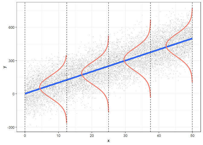
(3)번 방정식의 가장 우변을 살펴보자. 는 정규분포의 pdf이다. 이는 일반적인 OLS regression에서도 가정되는 사실인데, 아래와 같은 그림(출처)을 자주 접했을 것이다.
다음으로, 우변의 를 살펴보면, 다음과 같다.
여기서 으로 정규분포 pdf의 곱이고 는 정규분포인 사전분포를 가정했으므로 는 정규분포의 곱으로 이루어진 pdf라고 할 수 있다. 결론적으로, (3)번 방정식의 피적분항은 모두 정규분포의 곱으로 이루어진 pdf를 정규분포인 w에 관하여 marginalize하는 식이므로 좌변의 역시 정규분포의 pdf인 것을 알 수 있다. 참고로, Kilian Q. Weinberger교수님의 수업에서는 정규분포의 곱이 정규분포라는 논리를 사용하시는데, 이는 정확한 설명은 아닌듯 하다. 위에서 내가 언급한대로 정규분포의 곱은 정규분포는 아니고 어떤 정규분포에 proportional한 형태라는 사실을 확인했다.최종적으로 우리는 the posterior predictive distribution 가 정규분포를 따른다는 것을 확인했다.
참고 : (3)번 방정식의 가장 우변에 있는 를 데이터가 주어졌을 때, likelihood에 따라 모델(=)에 가중치(=)를 주고 모든 w에 대한 결과를 합한 거라고 해석하면 흥미로운 해석이 가능하다. 데이터에 비추어 보아 less likely한 weight를 갖는 모델에는 적은 가중치를 주고 더 나올 법한 weight를 갖는 모델에는 높은 가중치를 줘 가중평균을 구하는 방식으로 이해할 수 있다.
3. Fit the parameters and
가 정규분포를 따른다는 것을 확인하고 나면 이제부터 우리가 해야할 일은 이 정규분포의 평균과 공분산 행렬을 구하는 일로 축소된다. 즉, (3)번 방정식의 우변에 있는 적분 일체를 계산할 필요가 없는 것이다. 우리가 현재까지 확인한 사항은 다음과 같다.
여기서 는 간결함을 위해 0으로 가정하자. 사실 는 큰 관심사가 아니다. 를 0으로 만들기 위해 단순히 데이터의 label의 평균을 빼버리는 것과 같은 방식을 쉽게 취해줄 수 있다. 다음과 같이 좀 더 명시적으로 표현하겠다.
공분산 행렬 가 가져야할 성질들을 생각해보자. 우선 행렬은 positive semi definite이어야 한다. 또한, 행렬의 성분은 feature vector가 서로 가까운 값을 가질 수록 값은 1에 가까워지고 거리가 먼 독립적인 feature vector들 간에는 0의 값을 반환해야 한다.
여기서 공분산 행렬의 성분으로 kernel이 쓰일 여지가 생기게 된다. 예를 들어, rbf커널의 경우 위에서 말한 성질을 만족하며 간단한 형태이므로 아래에 등장하는 kernel(=)들에서는 단순성을 위해 rbf 커널을 가정한다. rbf 커널에 의한 공분산 행렬은 아래와 같이 명시된다. 두 feature vector간의 거리가 가까울 수록 1의 값을 갖고 멀어질 수록 0의 값을 갖는 것이 확인이 된다.
아래에서 활용될 기호를 정의하겠다.
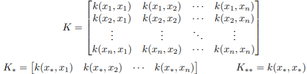
따라서, 와 같이 표현될 수 있다.
이렇게 표현하고 나면 (6)에서 도출한 결과를 통해 아래의 (8)을 유도할 수 있다.
multivariate normal distribution을 conditional normal distribution으로 바꿔주는 아래와 같은 공식이 성립한다고 알려져 있다.
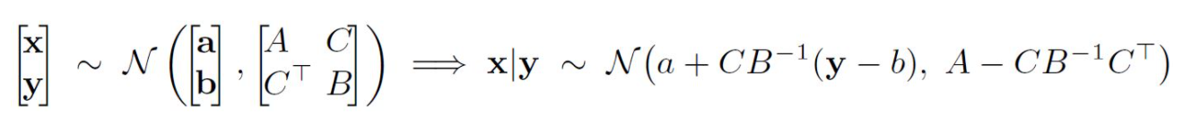
최종적으로 우리는 (8)번에 나타나있듯 the posterior predictive distribution의 확률분포를 모두 구하였다. 한 가지 흥미로운 점은 (8)번의 정규분포의 평균이 kernerl regression의 예측치와 동일하다는 점이다.
또한, Kilian Q. Weinberger교수님은 gaussian process regression의 가장 큰 장점은 uncertainty를 얘기할 수 있다는 점이라고 하였다. 우리는 단순히 예측값만 아는 것이 아니라 그 예측값의 확률 분포를 알기 때문에 uncertainty를 측정할 수 있다. 또한, 개인적으로는 이와 같이 uncertainty를 알 수 있다는 게 후에 bayesian optimization과 gaussian process가 연결되는 지점이라고 생각한다. bayesian optimization은 uncertainty가 더 많은 영역의 hyperparameter를 exploration하도록 설계될 수 있기 때문이다.
4. Connection to Bayesian Optimization
위의 그림(출처:https://ax.dev/versions/0.1.3/docs/bayesopt.html)은 Gaussian process와 bayesian optimization에 관해 학습을 하다 보면 자주 마주하게 되는 그림이다.
먼저 위에서 설명한 gaussian process의 연장선상에서 위 그림을 이해하기 위해서는 위에서 언급한 x들을 hyperparameter로 생각하고 y를 해당 hyper parameter에서의 모델 성능으로 생각할 필요가 있다.
예를 들어, RandomForest 모델에서 hyper parameter를 tuning하는 상황이라고 할 때, 와 같이 hyper parameter의 조합을 feature vector로 바라보고 이 조합의 hyper parameter에서의 모델 성능을 로 볼 필요가 있다.
Bayesian Optimization을 이해하는데 필수적인 개념인 Acquisition function에 대해 알아보자.
Acqusition function의 정의는 다음과 같다.
Acquisition functions are mathematical techniques that guide how the parameter space should be explored during Bayesian optimization.
They use the predicted mean and predicted variance generated by the Gaussian process model.
출처 : https://tune.tidymodels.org/articles/acquisition_functions.html
즉, Acqusition function은 hyper parameter space를 어떻게 탐색해나갈지 알려주는 technique인데, 그 과정에서 gaussian process에 의해 예측된 평균과 분산을 활용한다는 것이다.
hyper parameter를 탐색해 나갈 때는 아래와 같이 두 가지 전략이 고려될 수 있다. 아래 두 가지 전략은 서로 trade-off 관계에 있다.
<Bayesian Optimization에서 hyper parameter search시 고려되는 두가지 방향성>
-
exploitation : 현재 가장 좋은 성능이 확인된 parameter 주변을 search하는데 초점을 맞춘다.
-
exploration : uncertainty가 많이 남아있는 지역들을 search한다.
이 두가지 전략은 모두 나름대로 타당한 전략인데, exploitation의 경우 큰 함수값을 갖는 좋은 point들은 현재까지 확인된 point들 중에 가장 좋은값이 나온 곳 주변에 있을 가능성이 있기 때문이다. exploration의 경우 현재 정보가 없는 영역을 우리에게 알려준다. 따라서, 현재까지 관측한 point들보다 훨씬 좋은 point가 exploration한 곳에 있을 수 있다.
따라서, acquisition function은 이 두가지를 고려할 수 있게 고안되어야 하는데, 대표적인 acquisition function인 Expected Improvement에 대해 알아본다. Expected Improvement는 현재까지 관측된 hyper parameter의 조합 중 가장 좋은 성능을 보여주는 hyper parameter보다 더 가장 큰 성능의 개선을 가져다 줄 것으로 기대되는 hyper parameter를 찾아나서는 방법이다.
Expected Improvement의 공식은 다음과 같다.
이와 같은 expected improvement 산식은 closed form으로 부분적분을 이용해 풀면 아래와 같은 식이 된다는 것이 알려져있다.
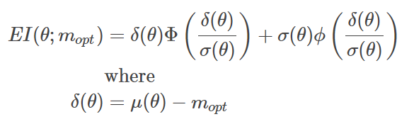
위의 Expected Improvement의 공식에서 항은 exploitation에 해당하는 항이고 항은 exploration에 해당하는 항이다. 다시 말해, 항은 새로 탐색할 parameter의 성능 평균이 현재까지의 가장 최고의 성능을 보여준 hyperparameter보다 얼마나 더 클지를 고려하는 항이다. 또한, 항은 새로 탐색할 parameter가 가지고 있는 uncertainty를 고려하는 항이다. 위에서 말했듯, exploitation과 exploration은 모두 합리적인 전략이라고 할 수 있는데, Expected Improvement의 경우 이 두 가지 전략이 고려되고 있음을 알 수 있다. 바로 위 GIF는 acquisition function을 Expected Improvement로 하고 있는데, GP estimate이 높은 곳과 uncertainty가 큰 곳을 위주로 탐색이 먼저 이루어지고 있음을 알 수 있다.
5. Practice with Bayesian Optimization
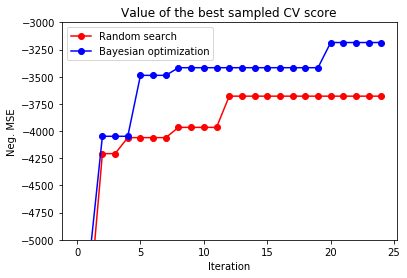
아래의 코드는 xgboost의 hyper parameter를 tuning할 때, randomized search를 했을 경우와 Bayesian Optimization을 적용했을 경우에 CV score가 어떻게 다르고, 몇번의 iteration만에 그 수준을 달성하는지를 비교할 수 있는 코드(출처:http://krasserm.github.io/2018/03/21/bayesian-optimization/)이다. 아래의 그래프를 통해 알 수 있듯이 Bayesian Optimization 방법이 훨씬 적은 iteration으로 더 높은 모델 성능을 보여주게 하는 hyper parameter를 찾는다는 점을 알 수 있다.
from sklearn import datasets
from sklearn.model_selection import RandomizedSearchCV, cross_val_score

from scipy.stats import uniform
from xgboost import XGBRegressor

# Load the diabetes dataset (for regression)
X, Y = datasets.load_diabetes(return_X_y=True)

# Instantiate an XGBRegressor with default hyperparameter settings
xgb = XGBRegressor()

# and compute a baseline to beat with hyperparameter optimization
baseline = cross_val_score(xgb, X, Y, scoring='neg_mean_squared_error').mean()


param_dist = {"learning_rate": uniform(0, 1),
              "gamma": uniform(0, 5),
              "max_depth": range(1,50),
              "n_estimators": range(1,300),
              "min_child_weight": range(1,10)}

rs = RandomizedSearchCV(xgb, param_distributions=param_dist,
                        scoring='neg_mean_squared_error', n_iter=25)

# Run random search for 25 iterations
rs.fit(X, Y);


bds = [{'name': 'learning_rate', 'type': 'continuous', 'domain': (0, 1)},
        {'name': 'gamma', 'type': 'continuous', 'domain': (0, 5)},
        {'name': 'max_depth', 'type': 'discrete', 'domain': (1, 50)},
        {'name': 'n_estimators', 'type': 'discrete', 'domain': (1, 300)},
        {'name': 'min_child_weight', 'type': 'discrete', 'domain': (1, 10)}]

# Optimization objective
def cv_score(parameters):
    parameters = parameters[0]
    score = cross_val_score(
                XGBRegressor(learning_rate=parameters[0],
                              gamma=int(parameters[1]),
                              max_depth=int(parameters[2]),
                              n_estimators=int(parameters[3]),
                              min_child_weight = parameters[4]),
                X, Y, scoring='neg_mean_squared_error').mean()
    score = np.array(score)
    return score

optimizer = BayesianOptimization(f=cv_score,
                                 domain=bds,
                                 model_type='GP',
                                 acquisition_type ='EI',
                                 acquisition_jitter = 0.05,
                                 exact_feval=True,
                                 maximize=True)

# Only 20 iterations because we have 5 initial random points
optimizer.run_optimization(max_iter=20)


y_rs = np.maximum.accumulate(rs.cv_results_['mean_test_score'])
y_bo = np.maximum.accumulate(-optimizer.Y).ravel()

print(f'Baseline neg. MSE = {baseline:.2f}')
print(f'Random search neg. MSE = {y_rs[-1]:.2f}')
print(f'Bayesian optimization neg. MSE = {y_bo[-1]:.2f}')

plt.plot(y_rs, 'ro-', label='Random search')
plt.plot(y_bo, 'bo-', label='Bayesian optimization')
plt.xlabel('Iteration')
plt.ylabel('Neg. MSE')
plt.ylim(-5000, -3000)
plt.title('Value of the best sampled CV score');
plt.legend();
6. 참고 자료
- https://www.cs.cornell.edu/courses/cs4780/2018fa/lectures/lecturenote15.html
- http://citeseerx.ist.psu.edu/viewdoc/summary?doi=10.1.1.363.7289&rank=88&q=stochastic
- https://arxiv.org/pdf/1505.02965.pdf
- https://arxiv.org/pdf/1807.02811.pdf
- https://greeksharifa.github.io/bayesian_statistics/2020/07/12/Gaussian-Process/
- https://ax.dev/versions/0.1.3/docs/bayesopt.html
- https://tune.tidymodels.org/articles/acquisition_functions.html
- http://krasserm.github.io/2018/03/21/bayesian-optimization/
- https://www.johndcook.com/blog/2012/10/29/product-of-normal-pdfs/
