Custom Dataset로 Yolov11 재학습하여 객체 감지 예측하기

짱아·2025년 8월 20일

로봇영상처리를 위한 AI모델 학습

목록 보기

9/9

https://colab.research.google.com/github/roboflow/notebooks/blob/main/notebooks/train-yolov8-object-detection-on-custom-dataset.ipynb#scrollTo=oe9vkEvFABbN

< 진행 절차 >
1. Data 준비하기 : Custom Dataset Dataset으로 Yolov11 재학습(Fine Tuning)하는 경우에는 Image / Annotation 으로 이루어진 Dataset 준비
- Roboflow에서 제공하는 Training Dataset을 이용하거나 Labeling Tool 을 이용하여 개발자가 직접 Labeling 시킨 Image / Annotation으로 이루어진 Training Dataset을 구축해야함
- Custom Dataset 구축시 이미지 데이터와 정답데이터는 확장자를 제외한 파일 이름은 동일해야하며 Yolov8에서 annotation 파일 즉 정답 파일의 확장자는 반드시 .txt 여야 함

1) Roboflow 에서 Aquarium Dataset (custom data) 다운로드
- Colab 으로 데이터셋 업로드 : Roboflow(https://public.roboflow.com/)에서 제공하는 Dataset 로드하기
2) yaml 파일 설정** (데이터셋 위치 알려주는 config file)
- 2-1) roboflow 에서 제공되는 data.yaml 파일 확인
- 2-2) custom data에 대한 yaml 파일 만들기
  Yolov8으로 Custom Data를 학습하기 위해서는 YAML 파일이 반드시 필요. YAML 파일에는 다음 정보를 포함해야함
  - 이미지와 정답이 저장되어 있는 디렉토리 정보
  - 인식하고 싶은 클래스 종류와 대응대는 각각의 이름
  - 형식 : 클래스번호 | x의 center 좌표|y의 center좌표| 너비 |높이
  - 전체 이미지의 width 와 height 값으로 나눈 비율값임

ultralytics 패키지 설치하기

pip install ultralytics

모델 객체 선언하고 학습하기

from ultralytics import YOLO
model = YOLO('yolo11.pt')  #  model = YOLO('yolo11n-seg.pt')
model.train(data='mydata.yaml', epochs=10)

객체 검출하기

results = model.predict(source='/content/test/')

결과 확인하기
결과 다운로드하기
학습된 모델 내보내기
웹캠에서 모델 사용하여 객체 검출하기

1. 데이터 준비하기(Custom Data 구축)

Roboflow : 컴퓨터 비전(딥러닝 기반 이미지 인식)을 쉽게 만들 수 있도록 도와주는 올인원 플랫폼
- 데이터셋, 모델 학습 및 관리, 다양한 공개 데이터, 모델 탐색 등 커뮤니티 활동 제공
Roboflow Universe – Rock-Paper-Scissors (SXSW)
- '가위 · 바위 · 보'를 탐지하는 객체 인식용 이미지 3,129장과 라벨 데이터셋

2. Roboflow 에서 Rock Paper Scissor Dataset (custom data) 다운로드

Public Dataset : https://universe.roboflow.com/roboflow-58fyf/rock-paper-scissors-sxsw
Download Dataset > Popular Download Formats - Select Format : Yolov11, show download code 선택 후 continue 버튼 클릭 > Your Download Code - Raw URL 탭에서 주소 복사하기

Roboflow 에서 직접 다운로드

!wget -O RockPaperScissors_Data.zip  https://universe.roboflow.com/ds/WeTWbWIpUy?key=4Rgbz2uHmy

압축파일 해제하기

!unzip -q /content/RockPaperScissors_Data.zip -d /content/RockPaperScissors_Data/

3. yaml 파일 설정 (데이터셋 위치 알려주는 config file)

YAML : 데이터 표현 양식의 한 종류
기본적으로 들여쓰기(indent)를 원칙으로하며 데이터는 Map(key-value)형식으로 작성

3-1. roboflow 에서 제공되는 data.yaml 파일 확인

# 셀 창에서 data.yaml 파일 확인하기. !cat 사용
!cat /content/RockPaperScissors_Data/data.yaml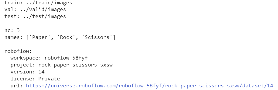

3.2 custom data에 대한 yaml 파일 만들기

# 파이썬에서 YAML 파일을 사용하기 위해 PyYAML 라이브러리 설치
!pip install PyYAML

파일 만들기

# yaml 파일을 학습이 가능하도록 경로 설정.
# key-value 데이터인 dict 데이터타입으로 data['train'], data['val'],
# data['nc'], data['names'] 에 넣어주는데,
# 가장 중요한 부분은 데이터 경로 설정임.

import yaml
# 디렉토리 정보, 클래스 이름(names), 클래스 수(nc) 지정하기
data = {
    'train': '/content/RockPaperScissors_Data/train/images',
    'val': '/content/RockPaperScissors_Data/valid/images',
    'test': '/content/RockPaperScissors_Data/test/images',
    'names': ['Papers', 'Rock', 'Scissors'],
    'nc': 3
}

# 데이터 경로와 클래스 정보를 저장하고 있는 딕셔너리 객체 data를
# YOLOv11 학습에 필요한 새로운 이름으로 저장
with open('/content/RockPaperScissors_Data/my.yaml', 'w') as f:
  yaml.dump(data, f)

확인

!cat /content/RockPaperScissors_Data/my.yaml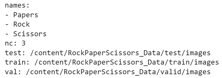

4. yolov11 사용을 위한 패키지 설치 및 가져오기

# YOLO 모델 사용 위한 패키지 설치하기
!pip install -q ultralytics

# 패키지 버전 확인하기
import ultralytics

ultralytics.checks()

import torch
torch.cuda.get_device_name(0)
torch.cuda.is_available()
print(torch.__version__)

# GPU가 사용 가능한지 확인하고, 사용 가능하면 CUDA를 사용하도록 설정
device = torch.device("cuda" if torch.cuda.is_available() else "cpu")
print(f"Using device: {device}")

5. 모델 객체 선언하고 학습하기

5-1. 모델 객체 선언하기

# YOLO 라이브러리 가져오기
from ultralytics import YOLO

# 'yolov11n.pt' 모델 선언하기 - 사전학습된 YOLO11 detection model 로드하기
model = YOLO('yolo11n.pt')

# Yolov11은 MS COCO 데이터 사전학습되어있어 MS COCO Dataset에 정의된 클래스 개수와 종류 확인할 수 있음(0~79)
print(type(model.names), len(model.names))

print(model.names)

5-2. 모델 학습하기 (자신의 만든 yaml파일 지정)

data: 데이터셋 설정 파일의 경로 지정- YAML 형식의 파일로, 훈련, 검증, 테스트 데이터 경로 및 클래스 수 정의
epochs: 훈련에 사용할 총 에포크 수 지정
patience: 모델 학습 중 개선이 없을 때 학습을 중단하기 전에 기다리는 에포크 수 지정
batch: 각 훈련 스텝에서 처리할 이미지의 수를 지정
imgsz: 입력 이미지의 해상도 정의(일반적으로 416, 512, 640과 같은 값이 사용)
optimizer: 사용할 최적화 알고리즘사 지정(일반적으로 SGD, Adam, AdamW와 같은 옵션을 사용)
lr0: 초기 학습률 지정
momentum: 모멘텀 지정
weight_decay: 가중치 감소(정규화)를 적용하는 값중 지정
warmup_epochs: 초기 학습률을 높이기 위해 사용할 웜업 에포크 수 지정
save: 훈련된 모델을 저장할지 여부 결정
project 및 name: 모델 가중치 및 훈련 로그를 저장할 프로젝트 폴더와 하위 폴더 이름을 지정

모델 학습하기

# 모델 학습하기 (자신의 만든 yaml파일 지정)
model.train(data = '/content/RockPaperScissors_Data/my.yaml',
            epochs = 10, patience = 2, batch = 32, imgsz = 416
)

굉장히 오래 걸린다.

# 커스텀 데이터로 학습하였기 때문에 클래수 수의 변경됨을 확인할 수 있음
print(type(model.names), len(model.names))

print(model.names)

결과: 클래스가 3개로 바뀐다.
<class 'dict'> 3
{0: 'Papers', 1: 'Rock', 2: 'Scissors'}

5-3. 테스트 이미지 데이터 생성 및 확인

# 테스트 이미지
from glob import glob

test_image_list = glob('/content/RockPaperScissors_Data/test/images/*')
test_image_list.sort()

for i in range(len(test_image_list)):
    print('i = ',i, test_image_list[i])

6.객체 검출 (Inference or predict)

객체 검출하기

result = model.predict(source='/content/RockPaperScissors_Data/test/images/', save = True)

7. 결과 확인하기

print(type(result), len(result))

7-1. 테스트 파일 이미지 이름과 예측 결과 출력해서 확인

import numpy as np
import os

for result in result:
    uniq, cnt = np.unique(result.boxes.cls.cpu().numpy(), return_counts=True)  # Torch.Tensor -> numpy
    uniq_cnt_dict = dict(zip(uniq, cnt))

    file_name = os.path.basename(result.path)
    print('\n',file_name)
    print('{class num : counts} =', uniq_cnt_dict,'\n')

    for i, c in enumerate(result.boxes.cls):
        class_id = int(c)
        class_name = result.names[class_id]
        confidence_score = result.boxes.conf[i]  # 예측 확률
        print(f'class num: {class_id:>2} , class name: {class_name :<13}, confidence: {confidence_score:.2f}')

결과는 아래와 같다.
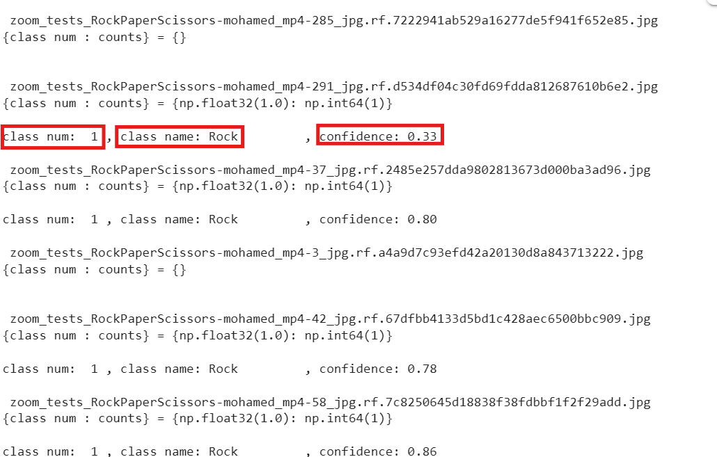
class_num, class_name, confidence(신뢰도)

7-2. 테스트 이미지 무작위로 50개만 선택해서 출력해보기

import random
from PIL import Image
from IPython.display import display
import os

# 이미지가 저장된 폴더 경로
image_dir = '/content/runs/detect/train2'

# 폴더 내 jpg 파일 목록 가져오기
jpg_files = [f for f in os.listdir(image_dir) if f.endswith('.jpg')]

# 무작위로 50개 선택 (파일 개수가 50개 미만이면 전부 선택)
sample_files = random.sample(jpg_files, min(50, len(jpg_files)))

# 선택된 파일 출력
for file_name in sample_files:
    file_path = os.path.join(image_dir, file_name)
    with Image.open(file_path) as img:
        display(img)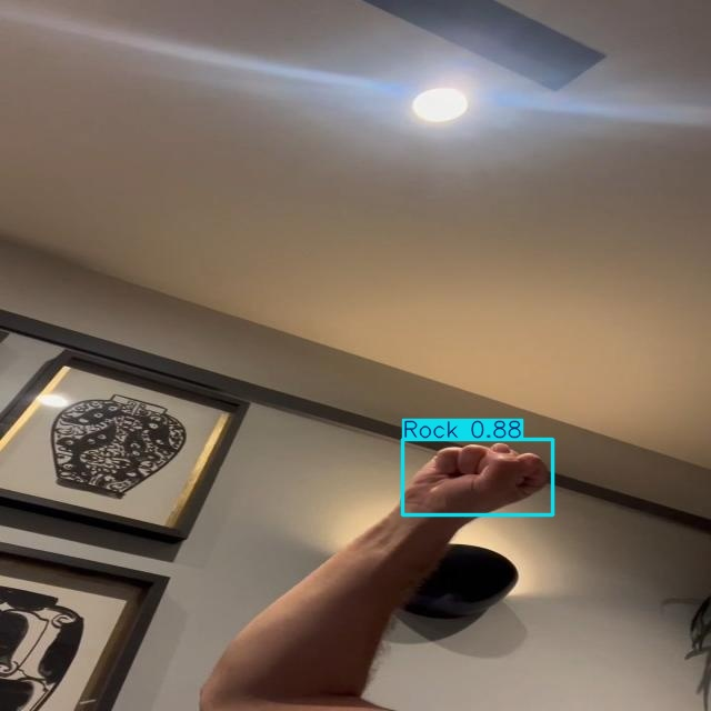

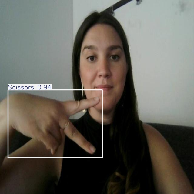
이런식으로 이미지들이 출력된다.

8. 평가

from PIL import Image
from IPython.display import display

# 오차행렬 이미지 경로
confusion_path = '/content/runs/detect/train/confusion_matrix.png'

# 이미지 열어서 출력
with Image.open(confusion_path) as confusion_image:
    display(confusion_image)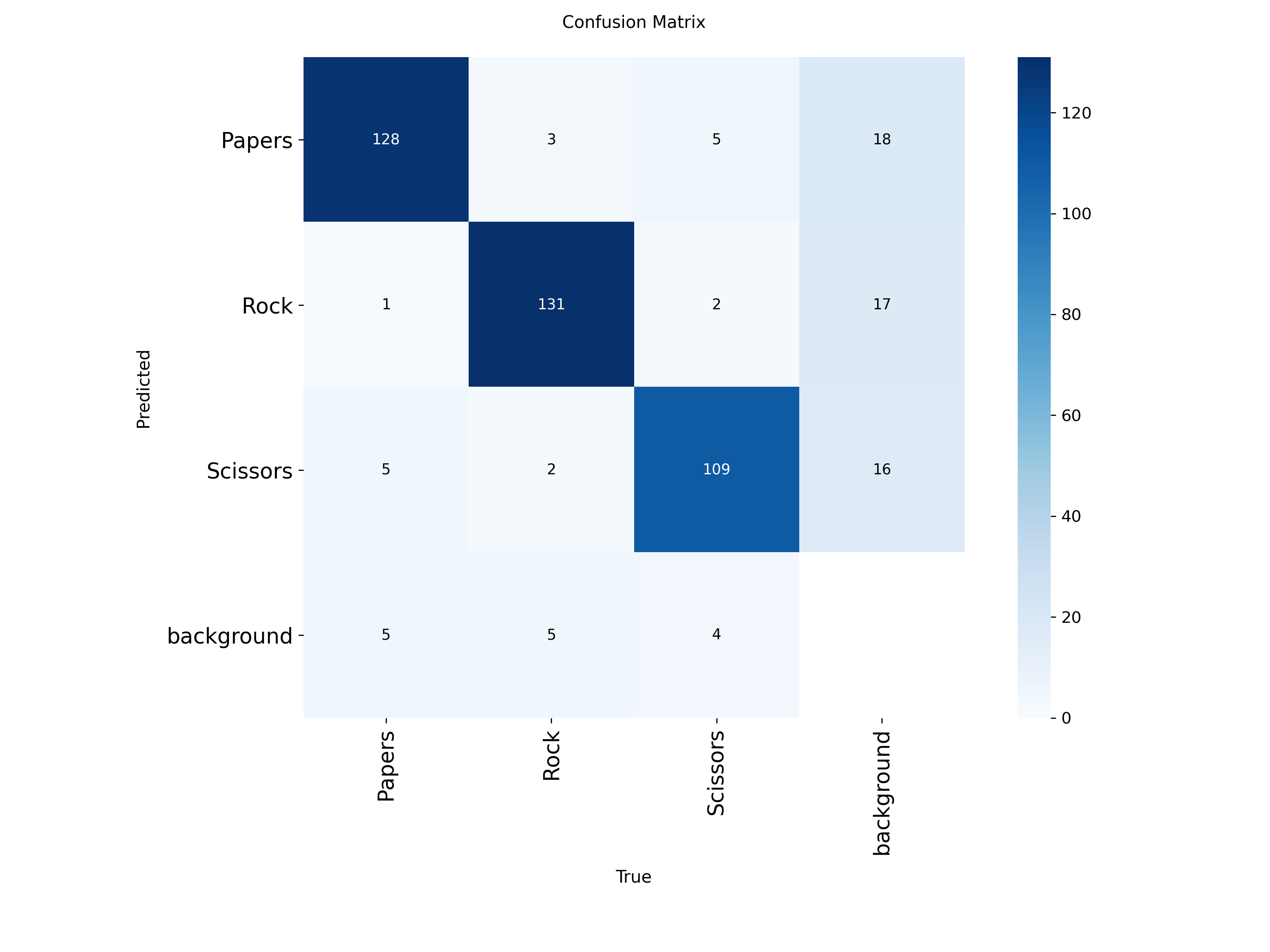

8-1. YOLO 모델 성능 평가 확인

mAP@0.5 : IoU 임계값 0.5일 때의 Mean Average Precision (객체 탐지 정확도 지표)

mAP@0.5:0.95 : IoU 임계값을 0.5 ~ 0.95까지 0.05 간격으로 바꿔가며 평균낸 mAP
→ 더 까다로운 기준, 일반적으로 이 값이 모델 성능의 표준 지표

Precision (정밀도) : 모델이 예측한 것 중 실제로 맞은 비율
(예측 → 정답 맞췄을 확률)

Recall (재현율) : 실제 정답 중에서 모델이 잘 찾아낸 비율
(실제 정답 → 모델이 얼마나 놓치지 않고 잡았는지)

Fitness : YOLO 내부에서 precision, recall, mAP를 종합적으로 고려해서 만든 통합 점수 (훈련 시 최적화 지표로 사용됨)

# 테스트 데이터셋에서 모델 평가
metrics = model.val(data='/content/RockPaperScissors_Data/my.yaml', split='test')

# mAP, Precision, Recall 값 출력

mAP_5 = metrics.results_dict['metrics/mAP50(B)']
mAP_5over = metrics.results_dict['metrics/mAP50-95(B)']
precision = metrics.results_dict['metrics/precision(B)']
recall = metrics.results_dict['metrics/recall(B)']

# Bounding box 기반의 mAP와 Precision, Recall을 종합적으로 고려하여 계산
fitness = metrics.results_dict['fitness']

print(f"mAP@0.5: {mAP_5:.4f}")
print(f"mAP@0.5:0.95: {mAP_5over:.4f}")
print(f"Precision: {precision:.4f}")
print(f"Recall: {recall:.4f}")
print(f"fitness: {fitness:.4f}")

# F1 Score 계산 (정밀도와 재현율이 모두 0이 아닐 때만 계산)
if precision + recall > 0:
    f1_score = 2 * (precision * recall) / (precision + recall)
else:
    f1_score = 0  # 정밀도와 재현율이 모두 0인 경우 F1 Score를 0으로 설정

print(f"F1 Score: {f1_score:.4f}")

짱아

짱아의 개발 일지

이전 포스트