안녕하세요. 이번 포스팅에서는 Transfer Learning, 즉 전이학습에 대해 공부해보는 시간을 갖도록 하겠습니다. 전이학습에 대한 자세한 내용은 링크로 남겨놓겠습니다.
간단하게 전이학습이 무엇인지에 대해 말씀드리겠습니다. 특정 이미지가 '개'인지, 아닌지에 대해 분류해야 하는 경우 일반적으로 우리는 방대한 양의 '개' 이미지로 모델을 학습시킵니다. 이 과정에서 오랜 시간이 걸리고 다양한 제약조건(데이터를 확보하거나 비용 문제)이 있을 수 있습니다. 이러한 문제를 해결하기 위해 사용되는 방법이 전이학습(=Transfer Learning)입니다.
ImageNet과 같은 방대한 양의 데이터를 기반으로 학습한 모델('개', '고양이' 등에 대한 동물 분류)이 있다고 했을 때, 우리는 이 모델을 가져와 우리에게 맞는 용도로 재학습 시킬 수 있습니다. 기존에 있던 모델을 'Pretrained model', 즉 사전학습된 모델이라고 부릅니다.
이 모델은 ImageNet의 데이터를 기반으로 학습된 모델입니다. 이 덕분에, 동물을 분류할 수 있는 사전학습된 모델은, 우리가 분류하려는 목적('개'인지 아닌지)에 대해 분류할 수 있게 됩니다. 사전학습된 모델의 가중치가 우리의 목적(이미지가 '개'인지 아닌지 분류)에도 유효하기 때문입니다.
전이학습에 대한 자세한 내용 및 코드는 아래에서 설명드리겠습니다.
톺아보다 : 틈이 있는 곳마다 모조리 더듬어 뒤지면서 찾다(순우리말).
Pytorch로 전이학습에 대한 코드실습을 해보겠습니다. 해당 코드는 파이토치 홈페이지의 내용을 바탕으로 작성하였음을 알려드립니다.
Step 01. 모델 설계
1.1 라이브러리 불러오기
from __future__ import print_function, division

import torch
import torch.nn as nn
import torch.optim as optim
from torch.optim import lr_scheduler
import numpy as np
import torchvision
from torchvision import datasets, models, transforms
import matplotlib.pyplot as plt
import time
import os
import copy

# interactive mode
plt.ion()
lr-scheduler - 1
lr_scheduler - 2
plt.ion()
1.2 데이터 불러오기
우리는 개미와 벌의 이미지를 분류하려고 합니다. 해당 데이터셋은 개미와 벌 각각에 대한 120여개의 training 이미지(총 240여개)와 150여개의 validation 이미지로 이루어져 있습니다. 이는 ImageNet의 데이터에서 가져온 극히 일부의 이미지이기에, 일반적으로 이러한 데이터로 모델을 학습시키기에는 부족한 감이 없지않아 있습니다. 따라서 이런 문제점을 개선하기 위해 앞서 말씀드린, 전이학습을 사용하는 것입니다.
# Data augmentation and normalization for training
# Just normalization for validation
# 딕셔너리를 사용하여 'train'과 'val'이라는 key 값에 transforms.Compose라는 value 값 정의.

data_transforms = {
    'train' : transforms.Compose([
                                  transforms.RandomResizedCrop(224),
                                  transforms.RandomHorizontalFlip(),
                                  transforms.ToTensor(),
                                  transforms.Normalize([0.485, 0.456, 0.406], [0.229, 0.224, 0.225])
    ]),

    'val' : transforms.Compose([
                                transforms.Resize(256),
                                transforms.CenterCrop(224),
                                transforms.ToTensor(),
                                transforms.Normalize([0.485, 0.456, 0.406], [0.229, 0.224, 0.225])
    ])
}
# Google Colab에서 사용하여 아래와 같은 경로로 저장하였습니다.
# 개인의 경로에 맞게 아래의 경로를 수정하시기 바랍니다.
data_dir = '/content/hymenoptera_data'
image_datasets = {x : datasets.ImageFolder(os.path.join(data_dir, x),
data_transforms[x])
for x in ['train', 'val']}
dataloaders = {x : torch.utils.data.DataLoader(image_datasets[x], batch_size = 4,
shuffle = True, num_workers = 4)
for x in ['train', 'val']}
dataset_sizes = {x : len(image_datasets[x]) for x in ['train', 'val']}
class_names = image_datasets['train'].classes
device = torch.device("cuda:0" if torch.cuda.is_available() else "cpu")데이터가 잘 저장되었는지 아래의 코드를 통해 확인해보겠습니다.
print("class_names : ", class_names)
print("\n")
print("datasets_sizes : ", dataset_sizes)
print("\n")
print("image_datasets : ", image_datasets)
# 출력결과
class_names : ['ants', 'bees']
datasets_sizes : {'train': 244, 'val': 153}
image_datasets : {'train': Dataset ImageFolder
Number of datapoints: 244
Root location: /content/hymenoptera_data/train
StandardTransform
Transform: Compose(
RandomResizedCrop(size=(224, 224), scale=(0.08, 1.0), ratio=(0.75, 1.3333), interpolation=bilinear)
RandomHorizontalFlip(p=0.5)
ToTensor()
Normalize(mean=[0.485, 0.456, 0.406], std=[0.229, 0.224, 0.225])
), 'val': Dataset ImageFolder
Number of datapoints: 153
Root location: /content/hymenoptera_data/val
StandardTransform
Transform: Compose(
Resize(size=256, interpolation=bilinear, max_size=None, antialias=None)
CenterCrop(size=(224, 224))
ToTensor()
Normalize(mean=[0.485, 0.456, 0.406], std=[0.229, 0.224, 0.225])
)}출력결과를 확인해보겠습니다. datasets_sizes에 244개의 train 이미지와 153개의 validation 이미지가 출력되는 것으로 보아, image_datasets에 이미지가 정상적으로 저장되어있음을 확인할 수 있습니다.
1.3 샘플 이미지 시각화
def imshow(inp, title = None) :
  # Imshow for Tensor
  inp = inp.numpy().transpose((1, 2, 0))
  mean = np.array([0.485, 0.456, 0.406])
  std = np.array([0.229, 0.224, 0.225])
  inp = std + inp * mean
  inp = np.clip(inp, 0, 1)
  plt.imshow(inp)

  if title is not None :
    plt.title(title)

# pause a bit so that plots are plotted
plt.pause(0.001)

# Get a batch of training data
inputs, classes = next(iter(dataloaders['train']))

# Make a grid from batch
out = torchvision.utils.make_grid(inputs)

imshow(out, title = [class_names[x] for x in classes])
print("inputs : ", inputs)
print("\n")
print("out : ", out)
# 출력결과
inputs : tensor([[[[-0.4397, -0.4568, -0.4397, ..., -0.1828, -0.1828, -0.1999],
[-0.4397, -0.4226, -0.4226, ..., -0.1999, -0.1999, -0.2342],
[-0.4226, -0.4226, -0.4226, ..., -0.2342, -0.2513, -0.2684],
...,
[-0.6281, -0.6794, -0.7479, ..., -0.6794, -0.6623, -0.6452],
[-0.5767, -0.6623, -0.7308, ..., -0.6794, -0.6452, -0.5938],
[-0.5767, -0.6623, -0.6965, ..., -0.5938, -0.5767, -0.5424]],
[[-0.7752, -0.7927, -0.7752, ..., -0.5126, -0.5126, -0.5301],
[-0.7752, -0.7752, -0.7752, ..., -0.5301, -0.5301, -0.5651],
[-0.7577, -0.7752, -0.7752, ..., -0.5651, -0.5826, -0.6001],
...,
[-0.8277, -0.8978, -0.9503, ..., -1.0553, -1.0378, -1.0203],
[-0.8277, -0.8627, -0.9153, ..., -1.0553, -1.0378, -1.0203],
[-0.8277, -0.8627, -0.9153, ..., -1.0203, -0.9853, -0.9503]],
[[-0.8458, -0.8633, -0.8458, ..., -0.7238, -0.7238, -0.7413],
[-0.8458, -0.8458, -0.8458, ..., -0.7413, -0.7413, -0.7761],
[-0.8284, -0.8458, -0.8458, ..., -0.7761, -0.7936, -0.8110],
...,
[-0.9853, -0.9853, -1.0027, ..., -1.2119, -1.1944, -1.1770],
[-0.9678, -1.0027, -1.0027, ..., -1.2119, -1.1944, -1.1596],
[-0.9678, -1.0027, -0.9853, ..., -1.1770, -1.1770, -1.1421]]],
[[[ 0.3652, 0.3138, 0.3994, ..., -0.8507, -0.8507, -0.7822],
[ 0.2111, 0.3309, 0.5193, ..., -0.8507, -0.7822, -0.7650],
[ 0.1939, 0.1768, 0.3823, ..., -0.8335, -0.8164, -0.8507],
...,
[-1.6213, -1.6213, -1.6555, ..., -1.5528, -1.5357, -1.5357],
[-1.6213, -1.6213, -1.6555, ..., -1.5528, -1.5699, -1.5357],
[-1.5870, -1.6384, -1.6555, ..., -1.5699, -1.5528, -1.6384]],
[[-1.1954, -1.2304, -1.1253, ..., -0.3025, -0.3375, -0.3550],
[-1.2654, -1.1078, -1.1253, ..., -0.3025, -0.3375, -0.3200],
[-1.2829, -1.1954, -1.3004, ..., -0.3200, -0.3025, -0.2850],
...,
[-1.2829, -1.2829, -1.3179, ..., -0.8978, -0.9153, -0.8803],
[-1.2829, -1.2829, -1.3004, ..., -0.9503, -0.9328, -0.9503],
[-1.2479, -1.3004, -1.3004, ..., -1.0028, -0.9678, -1.0203]],
[[-1.6999, -1.7870, -1.8044, ..., -1.6127, -1.6476, -1.6302],
[-1.7870, -1.7522, -1.7696, ..., -1.5953, -1.6127, -1.5953],
[-1.7522, -1.7696, -1.7696, ..., -1.6127, -1.6302, -1.6127],
...,
[-1.6302, -1.6302, -1.6302, ..., -1.2816, -1.3339, -1.2990],
[-1.6302, -1.6302, -1.6127, ..., -1.2816, -1.3513, -1.3687],
[-1.6302, -1.6476, -1.5953, ..., -1.3513, -1.3513, -1.3861]]],
[[[ 0.5878, 0.5878, 0.5878, ..., 2.0434, 2.0434, 1.9749],
[ 0.6049, 0.6392, 0.6221, ..., 2.0263, 2.0092, 1.9407],
[ 0.6392, 0.6563, 0.6563, ..., 2.0263, 2.0092, 1.9064],
...,
[-1.1418, -1.0390, -1.0219, ..., 0.8104, 0.8276, 0.8276],
[-1.0904, -1.0219, -1.0048, ..., 0.8447, 0.8618, 0.8618],
[-1.0390, -1.0219, -1.0048, ..., 0.8447, 0.8618, 0.8618]],
[[-0.6702, -0.6702, -0.6702, ..., 1.8859, 1.8508, 1.7283],
[-0.6877, -0.6527, -0.6702, ..., 1.8683, 1.8158, 1.6933],
[-0.6527, -0.6352, -0.6352, ..., 1.8333, 1.7983, 1.6583],
...,
[-1.2129, -1.1253, -1.0903, ..., 0.0476, 0.0651, 0.0651],
[-1.1604, -1.0903, -1.0728, ..., -0.0049, 0.0126, 0.0126],
[-1.1429, -1.0903, -1.0553, ..., -0.0399, -0.0224, -0.0224]],
[[-0.4275, -0.3927, -0.3927, ..., 2.2914, 2.2566, 2.1694],
[-0.4101, -0.3578, -0.3753, ..., 2.2740, 2.2391, 2.1346],
[-0.3753, -0.3404, -0.3404, ..., 2.2566, 2.2217, 2.0997],
...,
[-1.1247, -0.9678, -0.9330, ..., 0.0431, 0.0605, 0.0605],
[-1.0724, -0.9330, -0.8807, ..., 0.0256, 0.0431, 0.0431],
[-1.0201, -0.8981, -0.8807, ..., 0.0431, 0.0605, 0.0605]]],
[[[-1.6042, -1.5014, -1.5528, ..., -1.4158, -1.3815, -1.5357],
[-1.5870, -1.6042, -1.5357, ..., -1.4843, -1.4843, -1.4158],
[-1.4158, -1.4329, -1.3473, ..., -1.4672, -1.5014, -1.4158],
...,
[-1.7412, -1.7240, -1.5699, ..., -1.6727, -1.6213, -1.5699],
[-1.8097, -1.7412, -1.6727, ..., -1.7069, -1.6042, -1.6555],
[-1.7583, -1.6727, -1.7069, ..., -1.8268, -1.6727, -1.7412]],
[[-0.8803, -0.9153, -0.7752, ..., -0.6702, -0.7402, -0.6702],
[-0.8452, -0.8277, -0.8277, ..., -0.6702, -0.7227, -0.8102],
[-0.9328, -0.7752, -0.7227, ..., -0.7227, -0.7752, -0.8102],
...,
[-1.4230, -1.4580, -1.4930, ..., -1.3704, -1.3004, -1.1779],
[-1.3880, -1.3704, -1.3880, ..., -1.3529, -1.4230, -1.3004],
[-1.3704, -1.3529, -1.4230, ..., -1.3704, -1.3704, -1.3179]],
[[-1.4210, -1.2990, -1.4210, ..., -0.8633, -1.0724, -1.0201],
[-1.3513, -1.3339, -1.2816, ..., -0.9678, -1.1421, -1.1247],
[-1.4384, -1.3339, -1.2990, ..., -1.0550, -1.0550, -1.2293],
...,
[-1.4907, -1.4907, -1.4210, ..., -1.2467, -1.4036, -1.2816],
[-1.4907, -1.4733, -1.4210, ..., -1.1770, -1.2816, -1.3164],
[-1.4559, -1.4384, -1.4907, ..., -1.2467, -1.2119, -1.1944]]]])
out : tensor([[[ 0.0000, 0.0000, 0.0000, ..., 0.0000, 0.0000, 0.0000],
[ 0.0000, 0.0000, 0.0000, ..., 0.0000, 0.0000, 0.0000],
[ 0.0000, 0.0000, -0.4397, ..., -1.5357, 0.0000, 0.0000],
...,
[ 0.0000, 0.0000, -0.5767, ..., -1.7412, 0.0000, 0.0000],
[ 0.0000, 0.0000, 0.0000, ..., 0.0000, 0.0000, 0.0000],
[ 0.0000, 0.0000, 0.0000, ..., 0.0000, 0.0000, 0.0000]],
[[ 0.0000, 0.0000, 0.0000, ..., 0.0000, 0.0000, 0.0000],
[ 0.0000, 0.0000, 0.0000, ..., 0.0000, 0.0000, 0.0000],
[ 0.0000, 0.0000, -0.7752, ..., -0.6702, 0.0000, 0.0000],
...,
[ 0.0000, 0.0000, -0.8277, ..., -1.3179, 0.0000, 0.0000],
[ 0.0000, 0.0000, 0.0000, ..., 0.0000, 0.0000, 0.0000],
[ 0.0000, 0.0000, 0.0000, ..., 0.0000, 0.0000, 0.0000]],
[[ 0.0000, 0.0000, 0.0000, ..., 0.0000, 0.0000, 0.0000],
[ 0.0000, 0.0000, 0.0000, ..., 0.0000, 0.0000, 0.0000],
[ 0.0000, 0.0000, -0.8458, ..., -1.0201, 0.0000, 0.0000],
...,
[ 0.0000, 0.0000, -0.9678, ..., -1.1944, 0.0000, 0.0000],
[ 0.0000, 0.0000, 0.0000, ..., 0.0000, 0.0000, 0.0000],
[ 0.0000, 0.0000, 0.0000, ..., 0.0000, 0.0000, 0.0000]]])Step 02. 모델 학습 및 시각화
2.1 모델 학습하기
def train_model(model, criterion, optimizer, scheduler, num_epochs = 25)  :
  since = time.time()

# 모델 가중치(weights) 불러오기
  best_model_wts = copy.deepcopy(model.state_dict())
  best_acc = 0.0

  for epoch in range(num_epochs)  :
    print("Epoch {}/{}".format(epoch, num_epochs - 1))
    print("-" * 10)

    # Each epoch has a training and validation phase
    for phase in ['train', 'val'] :
      if phase == 'train' :
        model.train()   # Set model to training mode

      else :
        model.eval()    # Set model to evaluate mode

      running_loss = 0.0
      running_corrects = 0

      # Iterate over data.
      for inputs, labels in dataloaders[phase] :
        inputs = inputs.to(device)
        labels = labels.to(device)

        # zero the parameter gradients
        optimizer.zero_grad()

        # forward
        # track history if only in train
        with torch.set_grad_enabled(phase == 'train') :
          outputs = model(inputs)
          _, preds = torch.max(outputs, 1)
          loss = criterion(outputs, labels)

          # backward + optimize only if in training phase
          if phase == 'train' :
            loss.backward()
            optimizer.step()

        # statistics
        running_loss += loss.item() * inputs.size(0)
        running_corrects += torch.sum(preds == labels.data)

      if phase == 'train' :
        scheduler.step()

      epoch_loss = running_loss / dataset_sizes[phase]
      epoch_acc = running_corrects.double() / dataset_sizes[phase]

      print("{} Loss : {:.4f} Acc : {:.4f}".format(
        phase, epoch_loss, epoch_acc))

      # deep copy the model
      if phase == 'val' and epoch_acc > best_acc :
        best_acc = epoch_acc
        best_model_wts = copy.deepcopy(model.state_dict())

    print()

  time_elapsed = time.time() - since
  print("Training complete in {:.0f}m {:.0f}s".format(
      time_elapsed // 60, time_elapsed % 60))
  print("Best val Acc : {:4f}".format(best_acc))

  # load best model weights
  model.load_state_dict(best_model_wts)
  return model
with torch.set_grad_enabled(phase == 'train')
enumerate
2.2 예측한 모델 시각화하기
def visualize_model(model, num_images = 6) :
  was_training = model.training
  model.eval()
  images_so_far = 0
  fig = plt.figure()

  with torch.no_grad() :
    for i, (inputs, labels) in enumerate(dataloaders['val']) :
      inputs = inputs.to(device)
      labels = labels.to(device)

      outputs = model(inputs)
      _, preds = torch.max(outputs, 1)

      for j in range(inputs.size()[0]) :
        images_so_far += 1
        ax = plt.subplot(num_images // 2, 2, images_so_far)
        ax.axis("off")
        ax.set_title("predicted : {}".format(class_names[preds[j]]))
        imshow(inputs.cpu().data[j])

        if images_so_far == num_images :
          model.train(mode = was_training)
          return
    model.train(mode = was_training)
2.3 미세조정하기(=Finetuning)
# Finetuning the convnet

model_ft = models.resnet18(pretrained = True)
num_ftrs = model_ft.fc.in_features
# Here the size of each output sample is set to 2.
# Alternatively, it can be generalized to nn.Linear(num_ftrs, len(class_names)).

# resnet18 모델을 가져와 기존의 feature를, nn.Linear를 사용하여 2개의 feature(ants, bees)를 분류할 수 있게 변경.
model_ft.fc = nn.Linear(num_ftrs, 2)

model_ft = model_ft.to(device)

# 손실함수 정의
criterion = nn.CrossEntropyLoss()

# Optimizer 정의
# Observe that all parameters are being optimized
optimizer_ft = optim.SGD(model_ft.parameters(), lr = 0.001, momentum = 0.9)

# Decay LR by a factor of 0.1 every 7 epochs
exp_lr_scheduler = lr_scheduler.StepLR(optimizer_ft, step_size = 7, gamma = 0.1)
Step 03. 모델 학습 및 평가
3.1 모델 학습
model_ft = train_model(model_ft, criterion, optimizer_ft, exp_lr_scheduler, num_epochs = 25)# 출력결과
Epoch 0/24
----------
/usr/local/lib/python3.7/dist-packages/torch/nn/functional.py:718: UserWarning: Named tensors and all their associated APIs are an experimental feature and subject to change. Please do not use them for anything important until they are released as stable. (Triggered internally at /pytorch/c10/core/TensorImpl.h:1156.)
return torch.max_pool2d(input, kernel_size, stride, padding, dilation, ceil_mode)
train Loss : 0.5040 Acc : 0.7377
val Loss : 0.3973 Acc : 0.8693
Epoch 1/24
----------
train Loss : 0.4806 Acc : 0.8484
val Loss : 0.3875 Acc : 0.8366
Epoch 2/24
----------
train Loss : 0.5357 Acc : 0.7705
val Loss : 0.4966 Acc : 0.8105
...
(중략)
...
Epoch 23/24
----------
train Loss : 0.2226 Acc : 0.8975
val Loss : 0.2333 Acc : 0.9150
Epoch 24/24
----------
train Loss : 0.2859 Acc : 0.8852
val Loss : 0.2210 Acc : 0.9085
Training complete in 2m 14s
Best val Acc : 0.9281053.1.1 궁금한 사항 실험
# Train_model 함수에서 특정값들이 출력될 수 있게 코드 수정함
# forward
        # track history if only in train
        with torch.set_grad_enabled(phase == 'train') :
          outputs = model(inputs)
          print("outputs : ", outputs)
          print("\n")
          print("torch.max(outputs, 1) : ", torch.max(outputs, 1))
          print("\n")
          _, preds = torch.max(outputs, 1)
          print("\n")
          print("_, preds : ", _, preds)
          print("\n")
          loss = criterion(outputs, labels)

          # backward + optimize only if in training phase
          if phase == 'train' :
            loss.backward()
            optimizer.step()
# 출력결과(일부분)
Epoch 0/24
----------
outputs : tensor([[-0.0880, -0.3602],
[-0.5123, -0.2996],
[ 0.1827, -0.6169],
[-0.6210, -0.7068]], device='cuda:0', grad_fn=<AddmmBackward>)
torch.max(outputs, 1) : torch.return_types.max(
values=tensor([-0.0880, -0.2996, 0.1827, -0.6210], device='cuda:0',
grad_fn=<MaxBackward0>),
indices=tensor([0, 1, 0, 0], device='cuda:0'))
_, preds : tensor([-0.0880, -0.2996, 0.1827, -0.6210], device='cuda:0',
grad_fn=<MaxBackward0>) tensor([0, 1, 0, 0], device='cuda:0')
위의 출력된 결과를 분석해보겠습니다. 먼저 outputs을 보면, 4개의 행이 포함된 텐서가 출력된 것을 확인할 수 있습니다. 이는 batch_size = 4로 주었기 때문입니다. 이를 다른 숫자로 바꾸면 출력결과 역시 바뀝니다.
torch.max(outputs, 1)을 관찰해보면, outputs 텐서에서 각 행마다 최댓값이 저장되어있는 것을 확인할 수 있습니다. 이는 torch.max가 value와 index 둘 다를 저장하므로 위와 같은 결과를 얻을 수 있습니다. -0.0880과 -0.3602 중 큰 값은 -0.0880이므로 인덱스는 0이 저장되었습니다. 이런 과정을 총 4번(batch_size) 반복하여 저장합니다.
_, preds에서 preds에는 출력된 값의 맨 뒷부분인 tensor([0, 1, 0, 0]만 저장됩니다.
3.2 시각화
visualize_model(model_ft)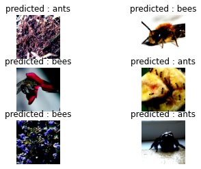
Step 04. FC layer를 제외한 나머지 parameter 동결
4.1 모델 학습 및 평가(동결된 모델)
model_conv = torchvision.models.resnet18(pretrained=True)
for param in model_conv.parameters():
    param.requires_grad = False

# Parameters of newly constructed modules have requires_grad=True by default
num_ftrs = model_conv.fc.in_features
model_conv.fc = nn.Linear(num_ftrs, 2)

model_conv = model_conv.to(device)

criterion = nn.CrossEntropyLoss()

# Observe that only parameters of final layer are being optimized as
# opposed to before.
optimizer_conv = optim.SGD(model_conv.fc.parameters(), lr=0.001, momentum=0.9)

# Decay LR by a factor of 0.1 every 7 epochs
exp_lr_scheduler = lr_scheduler.StepLR(optimizer_conv, step_size=7, gamma=0.1)
model_conv = train_model(model_conv, criterion, optimizer_conv,
exp_lr_scheduler, num_epochs=25)# 출력결과
Epoch 0/24
----------
train Loss : 0.5879 Acc : 0.7049
val Loss : 0.3701 Acc : 0.8366
Epoch 1/24
----------
train Loss : 0.5626 Acc : 0.7131
val Loss : 0.2810 Acc : 0.9085
Epoch 2/24
----------
train Loss : 0.5619 Acc : 0.7541
val Loss : 0.2008 Acc : 0.9346
...
(중략)
...
Epoch 23/24
----------
train Loss : 0.3277 Acc : 0.8402
val Loss : 0.2132 Acc : 0.9412
Epoch 24/24
----------
train Loss : 0.3313 Acc : 0.8607
val Loss : 0.1757 Acc : 0.9412
Training complete in 1m 34s
Best val Acc : 0.967320위의 결과(FC 레이어만 학습)와 이전의 결과(모든 layer 학습)를 비교해보면, Best val Acc가 위의 결과가 0.967320으로 더 높은 것을 확인할 수 있습니다. 즉, 모든 레이어를 학습시키는 것보다 마지막 레이어(FC layer)만 학습시켰을 때가 더 좋은 성능을 내는 것을 관찰할 수 있습니다.
visualize_model(model_conv)

plt.ioff()
plt.show()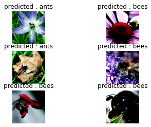
Reference