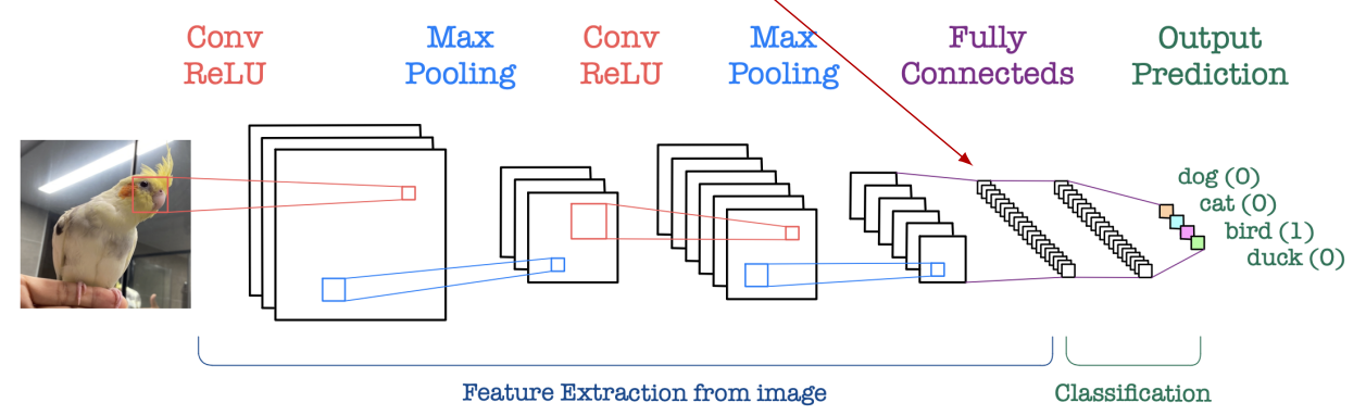
Convolutional Neural Network

Convolutional Neural Network (CNN)

CNN has great success in computer vision applications, especially in image classification,based on its shared weights using Convolution and translation invariance using Max pooling.

• Weight sharing makes it possible to handle input images of large sizes (huge input dimension). Translation invariance is an important property that is essential when dealing with image data.
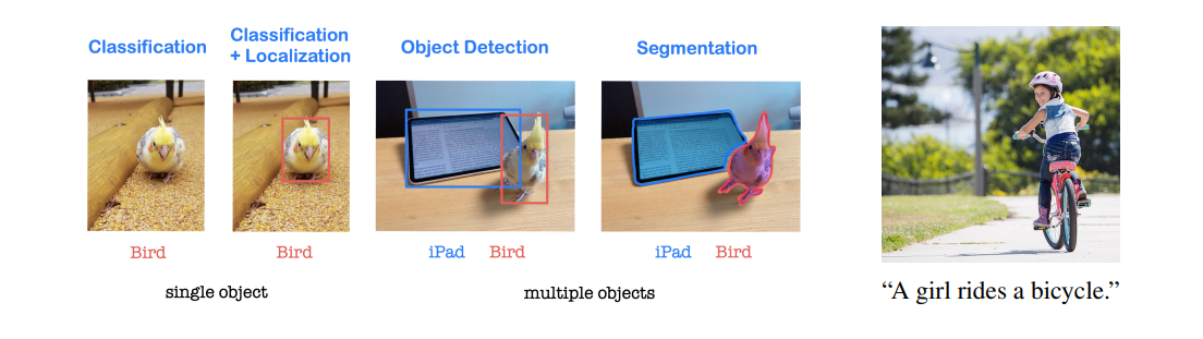
• Applications are image recognition, image classification, object detection and segmentation, and also CNN combined with LSTM is able to give image captioning.

CNN은 Convolutional Layer, Pooling Layer, Fully Connected Layer 등의 다양한 구성 요소로 이루어져 있습니다. Convolutional Layer는 입력 이미지와 학습 가능한 필터를 사용하여 이미지의 특징을 추출합니다. Max pooling은 특징 맵에서 가장 큰 값을 추출하여 공간 크기를 줄입니다. 이를 통해 이미지의 이동 불변성을 보장합니다.

Convolution과 Max pooling의 가중치 공유와 이동 불변성은 이미지의 지역적인 특징을 잘 추출할 수 있게 해줍니다. 예를 들어, 고양이의 얼굴을 인식하는 작업을 수행할 때, 이미지의 위치가 변해도 고양이의 얼굴 특징을 인식할 수 있습니다.

CNN은 이러한 특징들을 활용하여 이미지 데이터에 대한 다양한 작업을 수행하는 데 매우 효과적입니다. 그 결과, 컴퓨터 비전 분야에서 광범위하게 활용되고 있으며, 연구와 실제 응용에서 큰 성과를 거두고 있습니다.

Difficulties while using MLP to handle image data

• While using MLP to handle images with size $W×H$, the images are serialized (flattened) into vectors with very high dimension WH as inputs of the MLP network.

1. When the image becomes high-resolution, the serialized input data size increases rapidly, and so the number of parameters increases rapidly. (매개 변수 크기의 급격한 증가)
   If the image size is 1000×1000, then the serialized input size is 106, and so the number of parameters in the first layer is 1010 when the first hidden layer has 10000 nodes.

2. Due to the characteristics of the image, a specific pixel is spatially related to the surrounding pixels (지역성 locality), and this locality or spatial information is lost while serialization is performed to the image. (Weighted sum loses location information.)

3. For the new images obtained by small translations, transformations and scaling of an image, MLP considers them as totally different input data (no relation between them). This causes huge amount of training time for input images obtained by data augmentations (crop, shift, noise, rotate, scaling, etc).

MLP는 이미지 데이터를 처리하는 데 어려움을 겪으며, 이러한 문제를 극복하기 위해 CNN (합성곱 신경망)이나 다른 이미지 처리에 특화된 모델들이 주로 사용됩니다. CNN은 이미지의 공간적 특성을 유지하면서 효과적으로 특징을 추출할 수 있고, 가중치 공유와 풀링을 통해 매개 변수의 크기를 효율적으로 관리할 수 있습니다. 이를 통해 MLP에 비해 더 나은 성능을 얻을 수 있습니다.

CNN architecture

• LeCun creates the first CNN LeNet for character recognitions at 1998.
• AlexNet which is ILSVRC 2012 winner has similar structure as LeNet.

LeNet과 AlexNet의 주요 구성 요소
∗ Convolution (shared weights, dimension reduction)
∗ Nonlinearity (ReLU)
∗ Max pooling (translation invariance, dimension reduction for FC layer)
∗ Fully connected layer (classification)

Convolution: 합성곱은 이미지의 공간 정보를 활용하여 특징을 추출하는 역할을 합니다. 합성곱은 가중치를 공유하고 입력 데이터를 작은 필터로 슬라이딩하면서 특징 맵을 생성합니다. 이를 통해 공간적인 특징을 인식할 수 있으며, 가중치 공유로 인해 파라미터 수를 줄일 수 있습니다.

Nonlinearity: 비선형 함수인 ReLU(Rectified Linear Unit)는 합성곱과 풀링 레이어 사이에서 사용됩니다. ReLU는 입력값이 양수인 경우에는 그대로 전달하고, 음수인 경우에는 0으로 변환하여 비선형성을 도입합니다. 이를 통해 네트워크는 비선형 특징을 학습할 수 있습니다.

Max pooling: Max pooling은 특징 맵의 크기를 줄이는 과정입니다. 특정 영역에서 최대값을 추출하여 해당 영역의 대표값으로 사용합니다. 이를 통해 공간적 변동성을 감소시키고, 불필요한 정보를 제거하여 계산 비용을 줄이고 추상화된 특징을 유지합니다.

Fully connected layer: Fully connected layer는 최종적인 분류를 수행하는 역할을 합니다. 이 레이어는 전체 특징 맵을 1차원 벡터로 변환하여 입력으로 받고, 가중치와 편향을 활용하여 클래스를 분류합니다.

LeNet과 AlexNet은 합성곱과 풀링 레이어의 조합을 통해 공간적인 특징을 추출하고, 비선형성을 도입하여 복잡한 패턴을 학습할 수 있게 됩니다. 이후 이러한 아키텍처는 컴퓨터 비전 분야에서 큰 성과를 거두면서 다양한 CNN 모델의 기반을 마련하게 되었습니다.

Input image

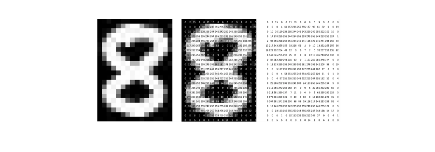
• Every input image can be represented as a matrix of pixel values.
• A color image has three RGB channels which are three 2d-matrices stacked together, each having pixel values in the range 0 to 255 for example.
• A grayscale image has one channel which is a single 2d-matrix each having pixel values in the range 0 (black) to 255 (white).

이러한 이미지 표현은 컴퓨터 비전 작업에서 매우 중요합니다. 이 픽셀 값 행렬을 입력으로 받아 다양한 이미지 처리 기법을 적용할 수 있습니다. 합성곱 신경망(CNN)에서는 이러한 이미지 표현을 활용하여 공간적인 특징을 추출하고, 패턴을 학습하며, 이미지를 분류, 인식 또는 다른 작업에 활용할 수 있습니다. 이를 통해 컴퓨터 비전 시스템은 컬러 이미지와 그레이스케일 이미지를 처리하고 분석하는 데에 큰 성과를 거두고 있습니다.

Convolution

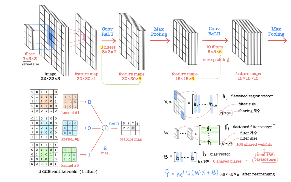
• Convolution layer as the core of CNN performs feature extraction by using filters while preserving spatial relationships between neighboring pixels (depending on kernel sizes).
• Convolution: multiplying elementwise by filters and summing the multiplication outputs.
• Ex) $3×3$ kernel or $3×3×1$ filter (9 shared weights sharing 12 times) acts on a $5×6$ input image and outputs a $3×4$ feature map in case of 1 input channel and 1 output feature map.

합성곱(Convolution)은 CNN의 핵심인 합성곱 레이어에서 수행되며, 필터를 사용하여 특징을 추출하면서 이웃하는 픽셀들 사이의 공간적인 관계를 유지합니다 (커널 크기에 따라 다릅니다).

합성곱은 각 픽셀에 필터를 적용하여 원소별로 곱한 후, 이 곱셈 결과를 모두 더하는 과정을 의미합니다. 예를 들어, $3×3$ 크기의 커널 또는 $3×3×1$ 크기의 필터(9개의 공유 가중치를 12번 공유)가 1개의 입력 채널과 1개의 출력 특징 맵을 가진 $5×6$ 크기의 입력 이미지에 작용한다면, $3×4$ 크기의 특징 맵이 출력됩니다.

이 과정을 통해 합성곱은 입력 이미지에서 지역적인 패턴이나 특징을 추출합니다. 필터는 작은 영역에서 특정한 패턴을 감지하도록 학습되며, 합성곱 연산을 통해 입력 이미지를 슬라이딩하면서 이 패턴의 존재 여부를 확인합니다. 이렇게 함으로써 공간적인 특징을 인식하고, 이를 통해 이미지 분류, 객체 검출, 분할 등의 작업에 사용됩니다.

합성곱은 가중치를 공유하여 파라미터 수를 효과적으로 관리할 수 있으며, 이를 통해 계산 비용을 줄이고 모델의 일반화 능력을 향상시킬 수 있습니다. 또한, 합성곱은 이미지의 공간적인 구조를 유지하면서 특징을 추출합니다.

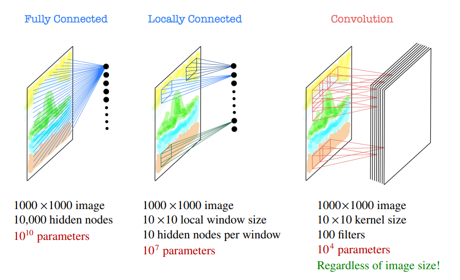
Why convolution?

합성곱(Convolution)은 이미지 처리에서 중요한 기법입니다. 다른 네트워크 구조와 비교하면서 설명해보겠습니다.

Fully Connected (완전 연결):
Fully Connected 네트워크는 이미지를 평탄화(flatten)하여 벡터 형태로 처리합니다. 예를 들어, $1000×1000$ 크기의 이미지를 입력으로 사용하고, $10,000$개의 은닉 노드를 가진 Fully Connected 네트워크를 사용한다면, 첫 번째 은닉층에는 $10^10$개의 파라미터가 필요하게 됩니다. 이미지 크기가 커질수록 매우 많은 파라미터가 필요하므로 계산적으로 매우 비효율적입니다.

Locally Connected (지역 연결):
지역 연결 네트워크는 이미지를 작은 지역 윈도우로 분할하여 처리합니다. 예를 들어, $1000×1000$ 크기의 이미지를 $10×10$ 크기의 로컬 윈도우와 $10$개의 은닉 노드를 가진 지역 연결 네트워크로 처리한다면, 각 윈도우마다 $10$개의 은닉 노드를 적용하여 $10^7$개의 파라미터가 필요하게 됩니다. 이미지 크기에 따라 파라미터 수가 증가하지만, Fully Connected에 비해 효율적입니다.

Convolution (합성곱):
합성곱 네트워크는 커널(필터)을 사용하여 이미지를 슬라이딩하면서 특징을 추출합니다. 예를 들어, $1000×1000$ 크기의 이미지에 $10×10$ 크기의 커널과 $100$개의 필터를 사용한다면, 총 $10^4$개의 파라미터가 필요하게 됩니다. 이미지 크기에 상관없이 커널 크기와 필터 수에 따라 파라미터 수가 결정되며, 다른 방법들에 비해 매우 효율적입니다.

이러한 이유로 합성곱은 이미지 처리에서 널리 사용되며, 이미지의 지역성을 유지하면서도 파라미터 수를 효율적으로 관리할 수 있습니다. 합성곱은 이미지 인식, 분류, 객체 검출 등 다양한 작업에서 큰 성과를 거두고 있습니다.

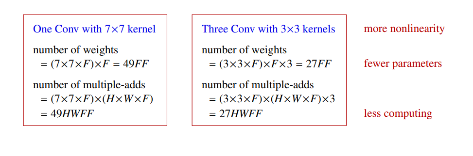
How to stack Convolution layers?

Three 3×3 Convolution layers give similar representational power
as a single 7×7 Convolution layer.

Compare convolutions on input channels of size $H × W × F (height × width × |channel|)$ with $F$ filters, stride $1$ and zero-padding, producing output feature maps of size $H × W × F$.

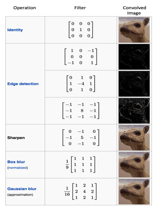
Filter matrix

Filter matrix
• Different values of the filter matrix produce different feature maps
for the same input image
• CNN learns the values of filters during training
although we specify the number of filters and
the filter size before training.
• The more filters, the more features are extracted
and the better the network will recognize patterns
in unseen images (test data).

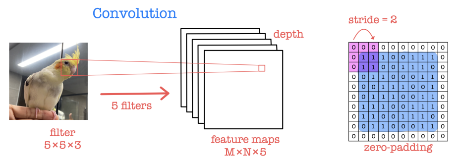
4 hyperparameters on Convolution layer

Size of a feature map is controlled by the following parameters that we specify.
• filters: number of filters (output feature maps)
• kernel size: size of kernel (convolution window: height × width)
• strides: distance between two successive kernel positions
• padding = ‘valid’ (no padding) or ‘same’ (padding with zeros to make the output with the same size as the input)

ReLU (nonlinearity)

• ReLU for nonlinearity has been used after every convolution operation.
• It is an elementwise operation (applied per pixel) and replaces all negative pixel values in the feature map by zero.

Max pooling

• Max pooling is for dimension reduction (downsampling) and translation invariance.
There is no learnable parameter in any of the pooling layers.
• It reduces the dimension of each feature map by taking
the largest element among every 2×2 window,
but retains the most important information.
Pooling is applied separately on each feature map.
• Max pooling makes the feature dimension smaller
and more manageable (eventually for FC layer).
• It introduces a translation invariance to small shifts,
distortions and scaling in the input image.
• This is very powerful since it can detect objects
in an image no matter where they are located.
Otherwise, we need huge amount of time training
much more images obtained by data augmentation.

Fully connected layer

• Fully connected layer is a traditional MLP that uses a softmax activation function
in the output layer.
Fully connected: each node in the previous layer is connected to every node in the next layer.
• The output from Convolutional and Max pooling layers represents high-quality features
of the input image.
• The number of nodes in FC layer is much smaller than the input dimension and so
manageable to compute.
• FC layer uses these high-quality features for classifying the input image into classes.

CNN architecture

• Convolution, ReLU and Max pooling layers are the basic block of CNN.
• All together extract useful features from inputs, introduce nonlinearity and reduce dimension,
while making the features somewhat invariant to shifts, distortions and scaling.
• Some of the best performing CNN have tens of Convolution and Max pooling layers.
It is not necessary to have a Max pooling layer after every Convolution layer.
• Fully connected layer acts as a classifier.

1×1 filters

It increases nonlinearity without affecting receptive field.

• 1×1 필터는 수용 영역을 변경하지 않으면서도 비선형성을 증가시키는 데 사용됩니다.

It is indeed Fully connected with weight sharing per feature map.
It is useful when we want to change the number of feature maps with minimal alteration.

네트워크의 용량을 효율적으로 관리하면서 표현력을 개선할 수 있는 방법.

1×1 필터를 사용하여 특징 맵의 차원을 줄이고, 다시 확장함으로써 병목 계층을 생성할 수 있습니다. 이를 통해 모델의 파라미터 수를 줄이고 연산 비용을 감소시키면서도 비선형성을 더욱 향상시킬 수 있습니다.

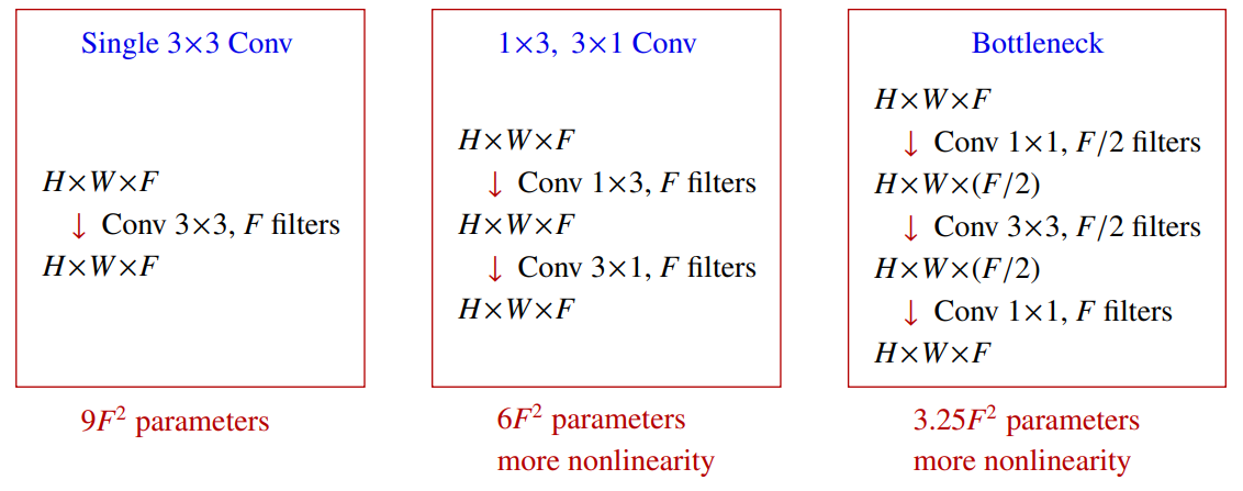
단일 3×3 합성곱은 가장 기본적인 형태의 합성곱 연산입니다. 3×3 커널을 사용하여 특징을 추출하고, 여러 개의 필터를 통해 입력 이미지의 다양한 특징을 학습할 수 있습니다.

1×3, 3×1 합성곱은 특정 방향에 대한 특징을 더 강조하는데 사용됩니다. 예를 들어, 1×3 합성곱은 수평적인 특징을, 3×1 합성곱은 수직적인 특징을 더욱 강조할 수 있습니다. 이를 통해 모델은 입력 이미지의 다양한 방향에서 특징을 추출할 수 있습니다.

병목 구조는 1×1 필터와 3×3 필터를 번갈아 가며 사용하는 구조입니다. 1×1 합성곱을 통해 입력 특징 맵의 차원을 줄이고, 이후 3×3 합성곱을 통해 더 많은 특징을 추출합니다. 마지막으로 다시 1×1 합성곱을 사용하여 차원을 확장하면서 비선형성을 높이는 효과를 얻습니다. 이러한 구조를 통해 모델은 보다 복잡한 특징을 학습할 수 있으며, 파라미터 수를 효과적으로 관리할 수 있습니다.

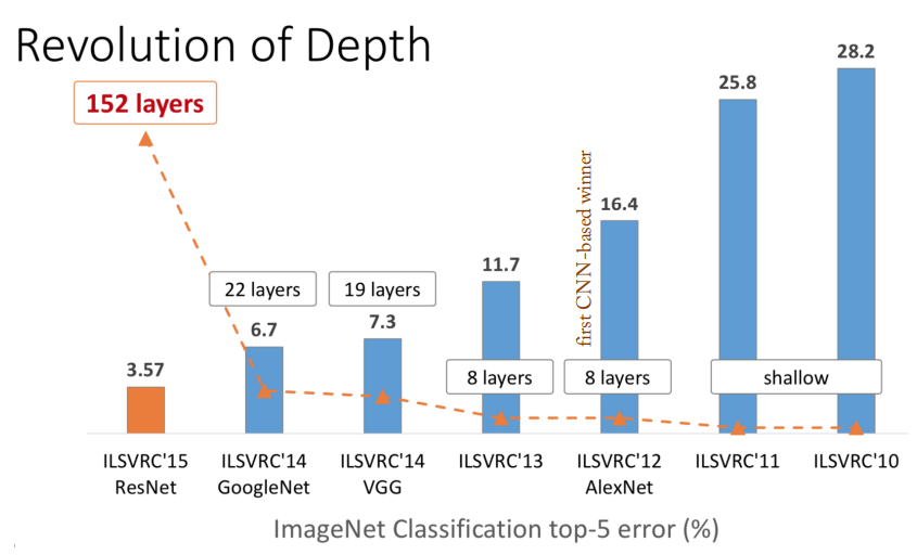
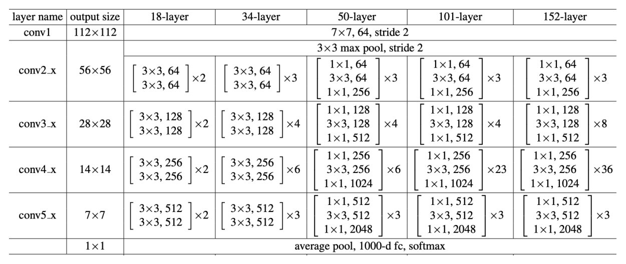
ResNet (Residual Network)

Deeper neural networks are more difficult to train due to the vanishing gradient problem!

Residual module

Residual $F(x)$ + identity shortcut $x$

• Simple design, but just deeper
• Few Max pooling
• No hidden FC, dropout
  
  

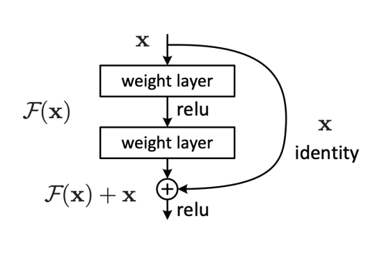
Importance of the identity mapping

• Very smooth forward pass
$x_K = x_k + \sum_{i=k}^{K-1}F(x_i)$
since $x_K = x_{K−1} + F(x_{K−1}) = x_{K−2} + F(x_{K−2}) + F(x_{K−1}) = · · · .$
⇒ Any $x_k$ is directly forward pass to any $x_K$, plus residual.
⇒ Any $x_K$ is an additive outcome, in contrast to multiplicative
($x_K=\prod_{i=k}^{K−1}W_ix_k.$)

• Very smooth backpropagation

• Deeper neural networks are more difficult to train due to the vanishing gradient problem.
This residual learning framework makes it easier to train much deeper networks by adding the identity mapping

Deep residual modules

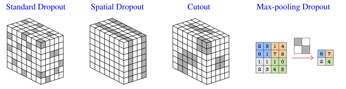
Dropout in Convolution layer

• Standard Dropout : If we randomly omit pixels then almost no information is removed as the omitted pixels are similar to their surroundings, so overfitting cannot be prevented.
• Spatial Dropout randomly drops out entire feature maps rather than individual pixels, bypassing dependency of adjacent pixels and promoting independence between feature maps.
• Cutout applies a random square mask directly over a larger region of each input image, unlike other common methods which apply dropout at the feature map level.
• Max-pooling Dropout applies dropout directly to Max pooling filter so that it minimizes the pooling of high activators.

• 표준 드롭아웃(Standard Dropout): 표준 드롭아웃은 픽셀을 무작위로 생략하여 정보의 손실을 거의 없게 합니다. 생략된 픽셀은 주변과 유사하기 때문에 과적합을 방지하는 데 도움이 되지 않습니다.

• 공간 드롭아웃(Spatial Dropout): 공간 드롭아웃은 개별적인 픽셀이 아닌 전체 특성 맵을 무작위로 생략합니다. 이로써 인접한 픽셀 간의 종속성을 피하고 특성 맵 간의 독립성을 촉진합니다.

• 컷아웃(Cutout): 컷아웃은 입력 이미지의 큰 영역에 무작위로 사각형 마스크를 적용합니다. 다른 일반적인 방법들은 특성 맵 수준에서 드롭아웃을 적용하는 반면, 컷아웃은 입력 이미지 자체에 직접 마스크를 적용합니다.

• 맥스 풀링 드롭아웃(Max-pooling Dropout): 맥스 풀링 드롭아웃은 드롭아웃을 맥스 풀링 필터에 직접 적용하여 높은 활성화를 갖는 요소들을 최소화합니다. 이를 통해 맥스 풀링이 강한 활성화를 유지하는 것을 방지할 수 있습니다.

이러한 드롭아웃 기법들은 신경망 모델에서 과적합을 줄이고 일반화 성능을 향상시키기 위해 사용됩니다. 각각의 기법은 고유한 특징을 가지고 있으며, 적절한 상황에서 사용될 수 있습니다.

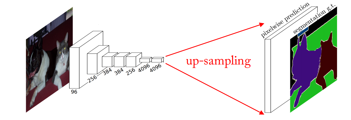
Up-sampling

Motivation: need a transformation going in the opposite direction of convolutions.
• Generating images involving up-sampling from low resolution to high resolution.
• Decoding layer of a convolutional auto-encoder.
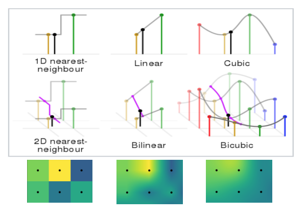
• Non-learnable interpolation methods
(nearest neighbor, bi-linear, bi-cubic)
which are like manual feature engineering.
• Learnable neural network up-samplings:

• Transposed convolution
• Fractionally-strided convolution

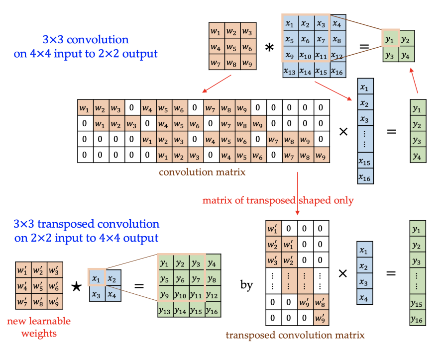
Transposed Convolution

• Convolution has the positional connectivity between the input values and the output values.
Ex) The top left values in the input channel affect the top left values of the output feature map.
Furthermore, it forms a many-to-one relationship like 3×3×F pixels (filter size) to 1 pixel.
• Transposed convolution is going backward of a convolution operation with the properties that
it has the similar positional connectivity and forms a one-to-many relationship.
• We can express a convolution operation using a convolution matrix, which is just
a rearranged matrix of weights to use a matrix multiplication to conduct convolutions.
• We similarly express a transposed convolution using a transposed convolution matrix,
whose layout is the transposed shape of the original convolution matrix,
but in which the actual weight values do not have to come from this convolution matrix.
The weights in the transposed convolution are learnable.

Fractionally-strided Convolution

• Similar to the standard convolution argument, it takes a convolution
after $n−1$ rows/columns between the input pixels (blue) are zero-padded.
• This makes the filter (kernel) move around at a slower pace on the input like $1/n$ strided.

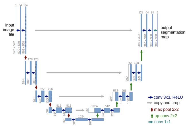
U-Net

U-Net is a U-shaped CNN used for object segmentation.

• Contracting path captures the context.
• Expanding path enables localization.

U-Net은 객체 분할(object segmentation)에 사용되는 U자 모양의 CNN이다.

수축 경로:
수축 경로는 입력 이미지를 다운샘플링하여 컨텍스트 정보를 캡처합니다. 이 과정에서 일반적으로 컨볼루션(Convolution), 풀링(Pooling), 활성화 함수(Activation function) 등을 사용하여 이미지의 특징을 추출합니다. 이를 통해 입력 이미지의 고수준 특징을 낮은 해상도로 압축하면서 컨텍스트 정보를 잘 보존합니다.

확장 경로:
확장 경로는 다운샘플링된 특징 맵을 업샘플링하고, 수축 경로에서 얻은 고수준 특징과 결합하여 객체의 정확한 위치를 예측합니다. 이를 통해 이미지의 해상도를 높이면서 객체의 세부 정보를 복원합니다. 업샘플링은 일반적으로 역컨볼루션(Deconvolution) 또는 전치 컨볼루션(Transpose Convolution)을 사용합니다.

To localize during up-sampling, high resolution features from the contracting path are combined to propagate context information to higher resolution layers.

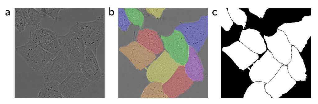
(a) input image of a cell
(b) manual ground truth segmentation
(c) generated output segmentation

U-Net은 객체 분할(object segmentation)에 사용되는 U자 모양의 합성곱 신경망(CNN)입니다. U-Net은 다음과 같은 특징을 가지고 있습니다.

U자 형태:
U-Net은 U자 형태의 아키텍처를 가지고 있습니다. 이 구조는 '수축 경로(contracting path)'와 '확장 경로(expanding path)'로 나누어져 있습니다. 수축 경로는 컨텍스트를 캡처하고, 확장 경로는 위치 정보를 활용하여 객체를 정확히 분할하는 데 도움을 줍니다.

스킵 연결:
U-Net에서는 확장 경로의 각 층에서 수축 경로에서 동일한 해상도의 특징 맵을 가져와 스킵 연결을 형성합니다. 이를 통해 고해상도 특징과 저해상도 특징을 결합함으로써 고해상도에서도 컨텍스트 정보를 활용할 수 있습니다. 스킵 연결은 정보의 유실을 방지하고 세밀한 분할을 가능하게 합니다.

U-Net은 객체 분할 작업에서 매우 효과적으로 작동하는 구조로 알려져 있으며, 의료 영상 분석 및 자율 주행차량 등 다양한 영역에서 사용되고 있습니다.