1. Instroduction
CNN은 computer vision 분야에서 이제는 빼놓을 수 없다. 트렌드는 높은 accuracy를 달성하기 위해 더 깊고 복잡한 network를 만드는 것이다. 그러나 size나 speed 측면에서는 더 효율적이진 않다.
이 논문에서는 효율적인 network architecture와, 모바일이나 임베디드 환경에 적합한 작은 모델을 위한 hyper parameters을 제시한다.
2. Prior Work
3. MobileNet Architecture
3.1 Depthwise Separable Convolutions
MobileNet은 depthwise separable convolution에 기반한다.
1. standard convolution into a depthwise convolution
2. pointwise convolution 1x1
각 채널에 하나의 필터를 적용한다. 그러고나서 pointwise convolution이 결합하게 된다.
depthwise separable convolution은 두개의 layer로 나뉜다.
-filtering ( standard convolution )
-combining ( pointwise )
이를통해 계산량고 모델 사이즈를 줄인다.
standard convolution layer
standard convolution layer은 DxDxM의 인풋을 가진다.
그리고 DxDxN 을 내보낸다.
M은 인풋 채널수, N은 아웃풋 채널수이다.
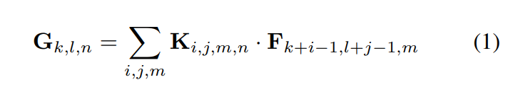
stride=1, padding을 가정하였을때 standard convolution 의 output featuremap이다.
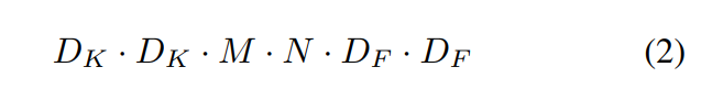
standard convolution은 위와 같은 계산 비용을 가진다.
계산 비용은 M,N, 커널사이즈 , feature map 사이즈에 의존한다.
MobileNet의 경우 output 채널 수와 커널 사이즈의 관계를 깨기 위해 depthwise separable convolution을 사용한다.
standard convolution의 경우 fitering과 combining에 영향을 받는다. filtering과 combination 단계가 depthwise separable convolution을 통해 분리될 수 있다.
Mobilenet은 두 layer( depthwise, pointwise )에 batchnorm과 ReLu 를 사용한다.
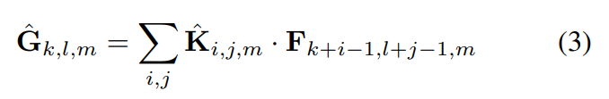
depthwise convolution
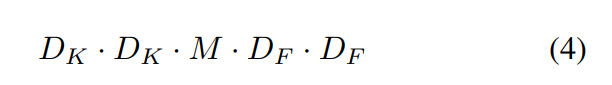
depthwise convolution은 위와 같은 계산비용을 가진다.
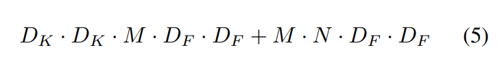
1x1 pointwise convolutio을 포함하면 이와 같다.
filtering과 combining의 단계를 통합함으로써 얻는 계산량의 감소
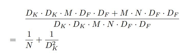
MobileNet은 3x3의 depthwise separable convolution을 사용하고 standard convolution보다 8~9배 낮은 계산량이다.
3.2 Network Structure and Training
Mobilenet은 full convolution으로 이루어진 첫번째 layer을 제외하고 depthwise separable convolution으로 이루어져있다.
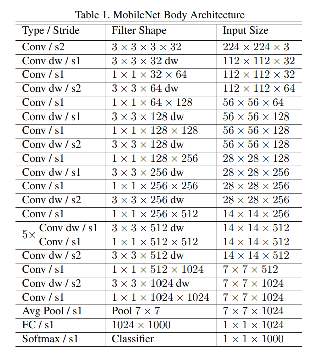
모든 layer가 batchnorm과 ReLU가 이어진다. ( 마지막 fc layer 제외 )
Mobilenet은 28 layer을 가진다.
네트워크가 작은 Mult-Adds(연산량)을 가지도록 하는 것은 간단하지 않다. 게다가 연산들이 효율적으로 실행되도록 하는 것이 중요하다.
예를들어 희소행렬이 dense행렬보다 일반적으로 계산이 빠르진 않다. Mobilenet 모델 구조는 모든 거의 모든 계산이 dense 1x1의 convolution이다. 이것은 GEMM function을 통해 연산될 수 있다. GEMM을 통해 실행되는 convolution은 보통 intial reordering을 요구하는데, 1x1 convolution의 경우엔 필요하지 않다.
Mobilenet 은 계산 시간의 95%를 1x1 convolution에 사용한다.
커다란 모델을 training 하는 것과 대비하여 적은 regularization, data augmentation이 사용된다. 왜냐하면 작은 모델은 overfitting의 문제가 적다.
depthwise flter에는 weigh decay가 매우 작거나 없어야 한다. ( 매우 적은 수의 파라미터가 있기 때문이다 )
3.3 Width Multiplier: Thinner Models
MobileNet 의 크기가 작고 적은 latency를 가지지만 그럼에도 불구하고 많은 특별한 경우 혹은 어플리케이션에서는 더 작고 빠른 모델을 요구한다.
이를 위해 매우 작은 파라미터 width multiplier을 소개한다. 이 파라미터는 각 레이어에서 균일하게 네트워크를 더 작게 만들어준다.

width multiplier 가 1, 0.75, 0.5, 0.25일때 기본 MobileNet의 경우 1의 값을 가지고 1보다 작아지면 더 작은 모델이 된다.
width multiplier을 통해 계산량을 줄이고, 파라미터의 수를 줄인다.
3.4 Resolution Multiplier: Reduced Representation

계산량을 줄이기 위한 두번째 파라미터는 resolution multiplier이다. 이것을 input 이미지와 모든 레이어의 internal representation에 적용한다.
resolution multiplier 이 1일때 기본 MobileNet이고, 1보다 작아지면 더 작은 모델이 된다.
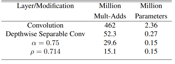
full convolution에 depthwise, a 파라미터, p파라미터를 차례대로 추가함에 따라 줄어드는 연산량과 파라미터의 변화를 볼 수 있다.
4. Experiments
4.1 Model Choices
4.2 Model Shrinking Hyperparameters
4.3 Fine Grained Recognition
4.4 Large Scale Geolocalization
4.5 Face Attribute
4.6 Object Detection
4.7 Face Embeddings
Conclution
지금까지 depthwise separable convolution에 기반한 MobileNets architecture을 제시하였다.
width multiplier과 resolution multiplier을 활용하여 더 작고 빠른 MobileNets를 만들었다.
그리고 MobileNets와 다른 모델들과 비교하였고, MobileNets이 큰 task에 적용될때 효과적이라는 것을 증명하였다.