
Titanic - Machine Learning from Disaster
Kaggle을 시작하게 되면 가장 먼저 혹은 쉽게 접할 수 있는 대회가 바로 Titanic 대회입니다. 저도 Kaggle이라는 데이터 분석 사이트를 접하게 되면서 처음 접했던 대회가 Titanic 이였고 다시 kaggle을 시작했기에 다시 한번 작성해보는 시간을 가지게 되었습니다.
결과적으로 Kaggle의 Public Leaderboard에는 0.79904로 2613등을 하게 되었으며 Public Leaderboard 기준으로는 상위 5% 정도로 생각됩니다. 데이콘에서도 Titanic 대회가 똑같이 존재해서 확인해보았는데, 0.778870의 accuracy를 확인할 수 있었습니다.
모델링 부분이 굉장히 부족하여 여러 노트북을 참고하였는데, A Data Science Framework: To Achieve 99% Accuracy 노트북을 정말 많이 참고하여 작성하게 되었습니다.
import os, sys

import glob
import zipfile

import numpy as np
import pandas as pd

import matplotlib.pyplot as plt
import seaborn as sns

import warnings
%matplotlib inlineplt.style.use('seaborn') # seaborn 스타일로 변환
sns.set(rc={'figure.figsize' : (15,7)})
plt.rc('font', family='AppleGothic')
plt.rc('axes', unicode_minus=False)
warnings.filterwarnings('ignore')0. 대회 설명
- 대회 : https://www.kaggle.com/c/titanic
- 주제 : predicts which passengers survived the trainanic shipwreck
- 문제 정의 : 어떤 특징의 승객이 살아남을 확률이 높을 것인가
- Data Description
- survival: 생존 여부 (0 = No, 1 = Yes)
- pclass: 티켓 등급 (1 = 1st, 2 = 2nd, 3 = 3rd)
- sex: 성별
- Age: 나이
- sibsp: 동행한 형재자매 / 배우자
- parch: 동행한 부모 / 자녀
- ticket: 티켓 번호
- fare: 요금
- cabin: 객실 번호
- embarked Port of Embarkation: 선착장 (C = Cherbourg, Q = Queenstown, S = Southampton)
1. Data Load
!kaggle competitions download -c titanictitanic.zip: Skipping, found more recently modified local copy (use --force to force download)os.listdir()['.DS_Store',
'Titanic.png',
'titanic.zip',
'.ipynb_checkpoints',
'data',
'Titanic.ipynb']unzip = zipfile.ZipFile('titanic.zip')
unzip.extractall(path = 'data')os.listdir('./data/')['test.csv',
'submission_soft.csv',
'train.csv',
'gender_submission.csv',
'submission_hard.csv']train = pd.read_csv(os.path.join('data', 'train.csv'))
test = pd.read_csv(os.path.join('data', 'test.csv'))train.head()| PassengerId | Survived | Pclass | Name | Sex | Age | SibSp | Parch | Ticket | Fare | Cabin | Embarked | |
|---|---|---|---|---|---|---|---|---|---|---|---|---|
| 0 | 1 | 0 | 3 | Braund, Mr. Owen Harris | male | 22.0 | 1 | 0 | A/5 21171 | 7.2500 | NaN | S |
| 1 | 2 | 1 | 1 | Cumings, Mrs. John Bradley (Florence Briggs Th... | female | 38.0 | 1 | 0 | PC 17599 | 71.2833 | C85 | C |
| 2 | 3 | 1 | 3 | Heikkinen, Miss. Laina | female | 26.0 | 0 | 0 | STON/O2. 3101282 | 7.9250 | NaN | S |
| 3 | 4 | 1 | 1 | Futrelle, Mrs. Jacques Heath (Lily May Peel) | female | 35.0 | 1 | 0 | 113803 | 53.1000 | C123 | S |
| 4 | 5 | 0 | 3 | Allen, Mr. William Henry | male | 35.0 | 0 | 0 | 373450 | 8.0500 | NaN | S |
train.describe()| PassengerId | Survived | Pclass | Age | SibSp | Parch | Fare | |
|---|---|---|---|---|---|---|---|
| count | 891.000000 | 891.000000 | 891.000000 | 714.000000 | 891.000000 | 891.000000 | 891.000000 |
| mean | 446.000000 | 0.383838 | 2.308642 | 29.699118 | 0.523008 | 0.381594 | 32.204208 |
| std | 257.353842 | 0.486592 | 0.836071 | 14.526497 | 1.102743 | 0.806057 | 49.693429 |
| min | 1.000000 | 0.000000 | 1.000000 | 0.420000 | 0.000000 | 0.000000 | 0.000000 |
| 25% | 223.500000 | 0.000000 | 2.000000 | 20.125000 | 0.000000 | 0.000000 | 7.910400 |
| 50% | 446.000000 | 0.000000 | 3.000000 | 28.000000 | 0.000000 | 0.000000 | 14.454200 |
| 75% | 668.500000 | 1.000000 | 3.000000 | 38.000000 | 1.000000 | 0.000000 | 31.000000 |
| max | 891.000000 | 1.000000 | 3.000000 | 80.000000 | 8.000000 | 6.000000 | 512.329200 |
train.nunique()PassengerId 891
Survived 2
Pclass 3
Name 891
Sex 2
Age 88
SibSp 7
Parch 7
Ticket 681
Fare 248
Cabin 147
Embarked 3
dtype: int64train.isnull().sum()PassengerId 0
Survived 0
Pclass 0
Name 0
Sex 0
Age 177
SibSp 0
Parch 0
Ticket 0
Fare 0
Cabin 687
Embarked 2
dtype: int642. EDA
2-1. label - Survived
# label - Survived  사망(0) / 생존(1) 비율
#  0, Dead / 1, Survived
f, ax = plt.subplots(1, 2, figsize=(15,8))
train['Survived'].value_counts().plot.pie(rot = 0, ax = ax[0])
ax[0].legend(['Dead', 'Survived'])
train['Survived'].value_counts().plot.bar(rot = 0, ax = ax[1])
ax[1].set_xticklabels(labels = ['Dead', 'Survived'])
plt.show()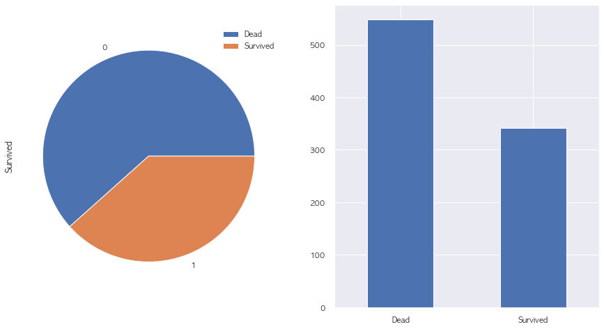
2-2. Feature distribution
# categorical feature에 대한 countplot
f, ax = plt.subplots(2,3, figsize = (20, 15))
columns = ['Survived', 'Pclass', 'Sex', 'SibSp', 'Parch', 'Embarked']
q = 0

for i in range(2):
    for j in range(3):
        fig = sns.countplot(x = train[columns[q]], ax = ax[i][j])
        q += 1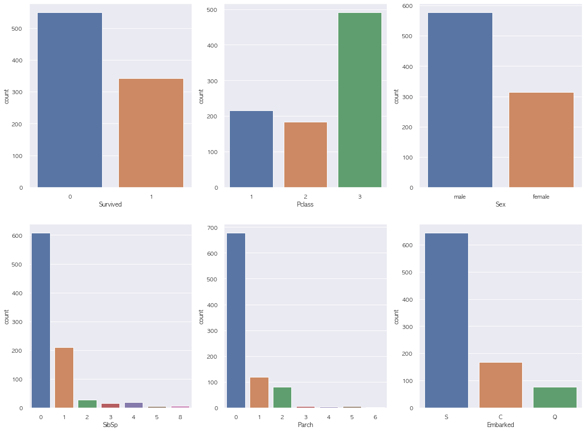
# continuous feature에 대한 countplot
f, ax = plt.subplots(2,1, figsize = (15, 10))
continuous_columns = ['Age', 'Fare']

train.Age.hist(bins = 70, ax = ax[0])
ax[0].set_title('Age distribution')

train.Fare.hist(bins = 70, ax = ax[1])
ax[1].set_title('Fare distribution')
plt.show()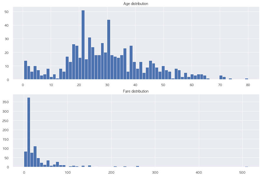
2-3. Sex
# 성별 사망 비율
f, ax = plt.subplots(1, 2, figsize=(15,8))
train.loc[train['Sex'] == 'male', 'Survived'].value_counts().sort_index().plot.bar(rot = 0, ax = ax[0], color = ['tab:blue', 'tab:orange'])
ax[0].set_title('male')
ax[0].set_xticklabels(['Dead', 'Survived'])
train.loc[train['Sex'] == 'female', 'Survived'].value_counts().sort_index().plot.bar(rot = 0, ax = ax[1], color = ['tab:blue', 'tab:orange'])
ax[1].set_title('female')
ax[1].set_xticklabels(['Dead', 'Survived'])
plt.show()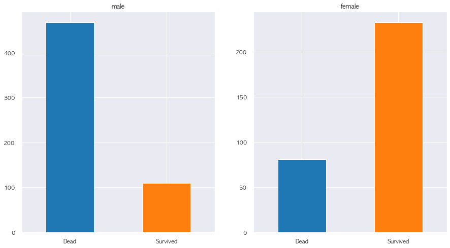
2-4. P_class
# P_class 별 생존여부
pd.pivot_table(train, index = 'Pclass', columns = 'Survived', values = 'Name', aggfunc='count', fill_value=0)
# pd.crosstab(train['Pclass'], train['Survived']) # 똑같은 결과| Survived | 0 | 1 |
|---|---|---|
| Pclass | ||
| 1 | 80 | 136 |
| 2 | 97 | 87 |
| 3 | 372 | 119 |
# Pclass가 3인 경우, 죽은 인원과 비율이 굉장히 많고 높음
# 보통 Pclasss는 남성인 경우가 많지만 생존된 비율은 여성이 더 높음
sns.countplot(data = train.loc[train['Pclass'] == 3], x = 'Sex', hue = 'Survived')
plt.show()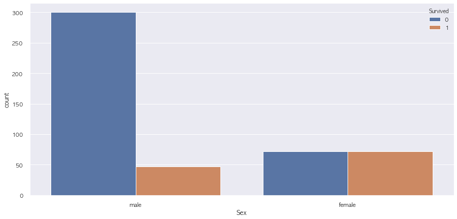
# Pclass $ sex 별 survived 분포
# Pclass 3->1 으로 갈수록 남성이 생존하는 비율이 높아지고
# Pclass 1 인 경우에는 여성이 사망하는 경우가 거의 없음
# 결론적으로, Pclass는 좀 더 고위층인 느낌인 들며 Survived(0/1)에 생각보다 영향을 많이 미치는 것 같음
sns.catplot(x = "Pclass", y = "Survived", hue = "Sex", row = "Sex", data = train,
            kind = "violin", split = True, height = 3, aspect = 4)
plt.show()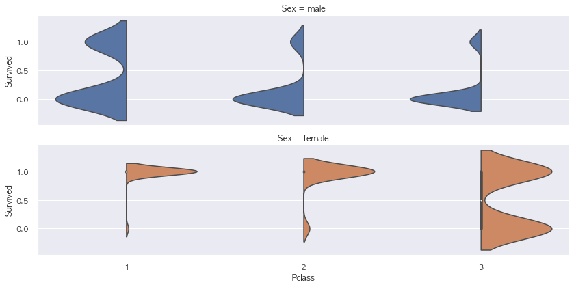
2-5. Age
# Pclass별 차이 확인
# Pclass & sex 별 나이 분포도
# Pclass 1->3 으로 갈수록 나이 분포가 점차 낮아지는 것을 확인 가능

f, ax = plt.subplots(3,2, figsize = (20, 15))
train.loc[(train['Pclass'] == 3) & (train['Sex'] == 'male'), 'Age'].hist(bins = 30, ax = ax[0][0])
train.loc[(train['Pclass'] == 3) & (train['Sex'] == 'female'), 'Age'].hist(bins = 30, ax = ax[0][1])
ax[0][0].set_title('Pclass 3 & male')
ax[0][1].set_title('Pclass 3 & female')

train.loc[(train['Pclass'] == 2) & (train['Sex'] == 'male'), 'Age'].hist(bins = 30, ax = ax[1][0])
train.loc[(train['Pclass'] == 2) & (train['Sex'] == 'female'), 'Age'].hist(bins = 30, ax = ax[1][1])
ax[1][0].set_title('Pclass 2 & male')
ax[1][1].set_title('Pclass 2 & female')

train.loc[(train['Pclass'] == 1) & (train['Sex'] == 'male'), 'Age'].hist(bins = 30, ax = ax[2][0])
train.loc[(train['Pclass'] == 1) & (train['Sex'] == 'female'), 'Age'].hist(bins = 30, ax = ax[2][1])
ax[2][0].set_title('Pclass 1 & male')
ax[2][1].set_title('Pclass 1 & female')

plt.suptitle('Pclass and Sex Age Distribution', fontsize = 20)

plt.show()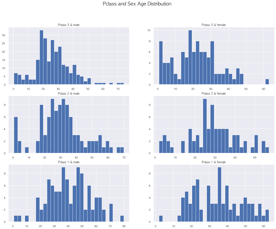
# boxplot 확인 결과 확실히 Pclass 낮을수록 연령대가 높음
sns.boxplot(x="Pclass", y="Age", data=train, whis=np.inf)
plt.show()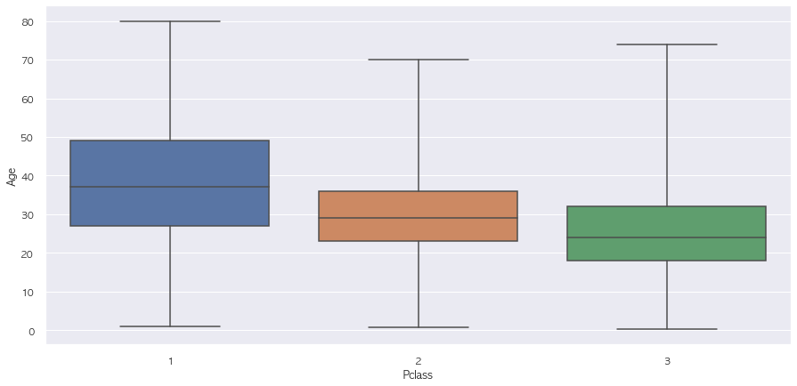
2-6. Cabin
# Cabin: 객실 번호 a small room where you sleep in a ship
# 선실의 종류를 의미하는 것 같기 때문에 Pclass와 같이 보면 좋을 것 같음
train['Cabin'].fillna('X').apply(lambda x : x[:1]).value_counts().plot.bar(rot = 0)
plt.show()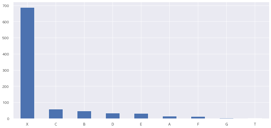
# NaN 제외 Cabin 분포
data = []
train.loc[train['Cabin'].notnull(), 'Cabin'].apply(lambda x : data.extend(x[:1]))
pd.Series(data).value_counts().sort_index().plot.bar(rot = 0)
plt.show()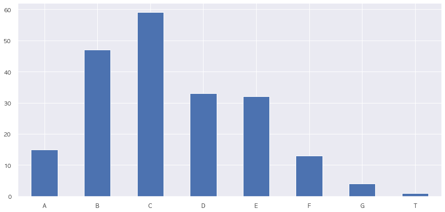
Pclass_cabin = train.loc[train['Cabin'].notnull(), ['Survived', 'Pclass', 'Cabin', 'Fare']]
Pclass_cabin['Cabin'] = Pclass_cabin['Cabin'].apply(lambda x : x[:1])
Pclass_cabin.head()| Survived | Pclass | Cabin | Fare | |
|---|---|---|---|---|
| 1 | 1 | 1 | C | 71.2833 |
| 3 | 1 | 1 | C | 53.1000 |
| 6 | 0 | 1 | E | 51.8625 |
| 10 | 1 | 3 | G | 16.7000 |
| 11 | 1 | 1 | C | 26.5500 |
# 흠.. 모집단이 너무 작아 확실한 결론을 내리기가 애매하지만..
# 일단 Pclass 1은 F, G, T 에는 거의 없음
pd.pivot_table(Pclass_cabin, index = 'Pclass', columns = 'Cabin', values = 'Survived', aggfunc = 'count')| Cabin | A | B | C | D | E | F | G | T |
|---|---|---|---|---|---|---|---|---|
| Pclass | ||||||||
| 1 | 15.0 | 47.0 | 59.0 | 29.0 | 25.0 | NaN | NaN | 1.0 |
| 2 | NaN | NaN | NaN | 4.0 | 4.0 | 8.0 | NaN | NaN |
| 3 | NaN | NaN | NaN | NaN | 3.0 | 5.0 | 4.0 | NaN |
# 확실히 Pclass가 높을수록 생존 가능성이 높다는 가설이 맞는것...같은...
# 그렇다면 비어있는 cabin에 대한 처리를 어떤식으로 할 수 있을까!
# 만약 Cabin 이 선실에 대한 의미이면 Fare(요금?)이랑 연관이 있지 않을까?!
pd.pivot_table(Pclass_cabin, index = 'Survived', columns = 'Cabin', values = 'Pclass', aggfunc = 'count')| Cabin | A | B | C | D | E | F | G | T |
|---|---|---|---|---|---|---|---|---|
| Survived | ||||||||
| 0 | 8.0 | 12.0 | 24.0 | 8.0 | 8.0 | 5.0 | 2.0 | 1.0 |
| 1 | 7.0 | 35.0 | 35.0 | 25.0 | 24.0 | 8.0 | 2.0 | NaN |
# 오오.. 확실히 Pclass 1의 Cabin의 fare가 높음
pd.pivot_table(Pclass_cabin, index = 'Pclass', columns = 'Cabin', values = 'Fare', aggfunc = np.mean)| Cabin | A | B | C | D | E | F | G | T |
|---|---|---|---|---|---|---|---|---|
| Pclass | ||||||||
| 1 | 39.623887 | 113.505764 | 100.151341 | 63.324286 | 55.740168 | NaN | NaN | 35.5 |
| 2 | NaN | NaN | NaN | 13.166675 | 11.587500 | 23.75000 | NaN | NaN |
| 3 | NaN | NaN | NaN | NaN | 11.000000 | 10.61166 | 13.58125 | NaN |
pd.pivot_table(Pclass_cabin, index = 'Survived', columns = 'Cabin', values = 'Fare', aggfunc = np.median)| Cabin | A | B | C | D | E | F | G | T |
|---|---|---|---|---|---|---|---|---|
| Survived | ||||||||
| 0 | 37.3896 | 42.7500 | 81.1625 | 43.5604 | 45.18125 | 7.65000 | 10.4625 | 35.5 |
| 1 | 35.5000 | 91.0792 | 89.1042 | 63.3583 | 39.82500 | 24.17915 | 16.7000 | NaN |
2-7. Fare
# Fare가 10 이하일 경우에는 F, G 랜덤 부여
# Fare가 10 초과 50 이하일 경우에는 A, D, E, T
# Fare가 50 초과일 경우에는 B, C
sns.boxplot(x = "Cabin", y = "Fare", data = Pclass_cabin.sort_values('Cabin'), whis = np.inf)
plt.show()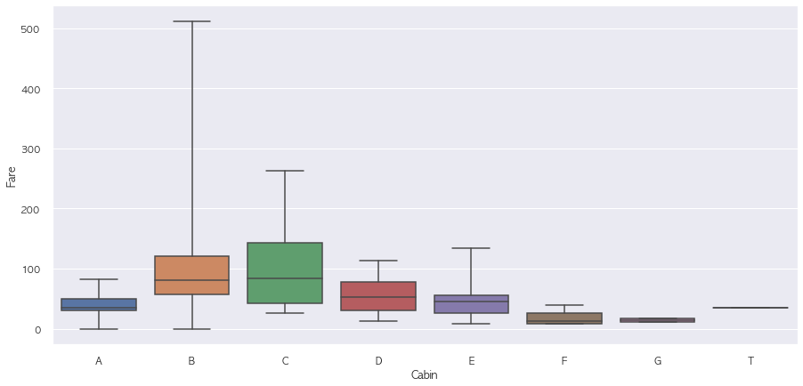
2-8. Name
# 이름에서 생존여부 차이를 알 수 있을까train.loc[(train['Name'].str.contains('Mr')) & (train['Name'].str.contains('Mrs') == False)]| PassengerId | Survived | Pclass | Name | Sex | Age | SibSp | Parch | Ticket | Fare | Cabin | Embarked | |
|---|---|---|---|---|---|---|---|---|---|---|---|---|
| 0 | 1 | 0 | 3 | Braund, Mr. Owen Harris | male | 22.0 | 1 | 0 | A/5 21171 | 7.2500 | NaN | S |
| 4 | 5 | 0 | 3 | Allen, Mr. William Henry | male | 35.0 | 0 | 0 | 373450 | 8.0500 | NaN | S |
| 5 | 6 | 0 | 3 | Moran, Mr. James | male | NaN | 0 | 0 | 330877 | 8.4583 | NaN | Q |
| 6 | 7 | 0 | 1 | McCarthy, Mr. Timothy J | male | 54.0 | 0 | 0 | 17463 | 51.8625 | E46 | S |
| 12 | 13 | 0 | 3 | Saundercock, Mr. William Henry | male | 20.0 | 0 | 0 | A/5. 2151 | 8.0500 | NaN | S |
| ... | ... | ... | ... | ... | ... | ... | ... | ... | ... | ... | ... | ... |
| 881 | 882 | 0 | 3 | Markun, Mr. Johann | male | 33.0 | 0 | 0 | 349257 | 7.8958 | NaN | S |
| 883 | 884 | 0 | 2 | Banfield, Mr. Frederick James | male | 28.0 | 0 | 0 | C.A./SOTON 34068 | 10.5000 | NaN | S |
| 884 | 885 | 0 | 3 | Sutehall, Mr. Henry Jr | male | 25.0 | 0 | 0 | SOTON/OQ 392076 | 7.0500 | NaN | S |
| 889 | 890 | 1 | 1 | Behr, Mr. Karl Howell | male | 26.0 | 0 | 0 | 111369 | 30.0000 | C148 | C |
| 890 | 891 | 0 | 3 | Dooley, Mr. Patrick | male | 32.0 | 0 | 0 | 370376 | 7.7500 | NaN | Q |
518 rows × 12 columns
# 이름 에서 찾을 수 있는 성별 및 결혼 여부
# 남자 기혼인 경우에 Survived 하지 못하는 경우가 더 많음
f, ax = plt.subplots(4,1, figsize = (17, 10))

train.loc[(train['Name'].str.contains('Mr')) & (train['Name'].str.contains('Mrs') == False), 'Survived'].value_counts().sort_index().plot.bar(ax = ax[0])
ax[0].set_title('Name(Mr) Survived')

train.loc[train['Name'].str.contains('Mrs'), 'Survived'].value_counts().sort_index().plot.bar(ax = ax[1])
ax[1].set_title('Name(Mrs) Survived')

train.loc[train['Name'].str.contains('Miss'), 'Survived'].value_counts().sort_index().plot.bar(ax = ax[2])
ax[2].set_title('Name(Miss) Survived')

train.loc[~train['Name'].str.contains('Mr|Miss|Mrs'), 'Survived'].value_counts().sort_index().plot.bar(ax = ax[3])
ax[3].set_title('Name(Not) Survived')

plt.show()
train['Agegroup'] = train['Age'].apply(lambda x : 'baby' if (x > 0) & (x < 10) else (
            'Child' if (x > 10) & (x <= 20) else(
            'Teenager' if (x > 20) & (x <= 40) else(
            'Young' if (x > 40) & (x <= 50) else(
            'Adult' if (x > 50) & (x <= 60) else(
            'Senior' if x > 60 else 'Unknown'
))))))pd.pivot_table(train, index = 'Survived', columns = 'Agegroup', values = 'Fare', aggfunc = 'count')| Agegroup | Adult | Child | Senior | Teenager | Unknown | Young | baby |
|---|---|---|---|---|---|---|---|
| Survived | |||||||
| 0 | 25 | 71 | 17 | 232 | 127 | 53 | 24 |
| 1 | 17 | 44 | 5 | 153 | 52 | 33 | 38 |
2-9. SipSp & Parch
# SipSp 는 Sibling(형제자매) + Spouse(배우자)
# Parch 는 Parents(부모) + Children(자녀)
# SipSp 와 Parch 로 동행 가족의 수를 보여주는 것 같음
train['family_cnt'] = train.apply(lambda x : x['SibSp'] + x['Parch'], axis = 1)pd.pivot_table(train, index = 'Survived', columns = 'Sex', values = 'family_cnt', aggfunc = np.mean)| Sex | female | male |
|---|---|---|
| Survived | ||
| 0 | 2.246914 | 0.647436 |
| 1 | 1.030043 | 0.743119 |
sns.boxplot(x = "Survived", y = "family_cnt", data = train, hue = 'Sex')
plt.show()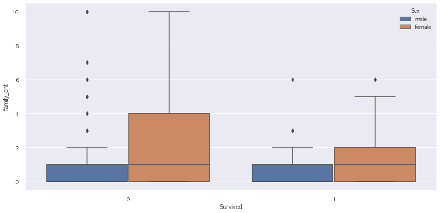
train.loc[train['family_cnt'] > 4, 'Survived'].value_counts()0 40
1 7
Name: Survived, dtype: int642-10. Embarked
sns.countplot(data = train, x = 'Embarked', hue = 'Survived')
plt.show()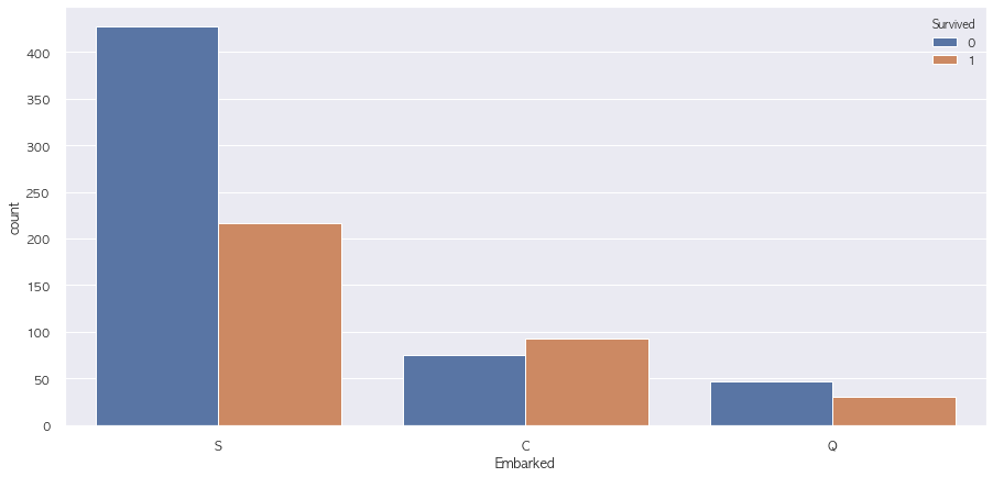
pd.pivot_table(train, index = 'Survived', columns = 'Embarked', values = 'family_cnt', aggfunc = 'count')| Embarked | C | Q | S |
|---|---|---|---|
| Survived | |||
| 0 | 75 | 47 | 427 |
| 1 | 93 | 30 | 217 |
3. Preprocessing
from sklearn.base import BaseEstimator, TransformerMixinclass preprocessing(BaseEstimator, TransformerMixin):
def fit(self, X, y = None):
return self
def transform(self, X, y = None):
# 나이 null값 채우기
temp = pd.pivot_table(X, index = 'Pclass', columns = 'Sex', values = 'Age', aggfunc = np.median)
for pclass, sex in X.loc[X['Age'].isnull(), ['Pclass', 'Sex']].drop_duplicates().values:
X.loc[(X['Age'].isnull()) & (X['Pclass'] == pclass) & (X['Sex'] == sex), 'Age'] = temp.loc[pclass, sex]
# 나이 그룹 피처 생성
X['Agegroup'] = X['Age'].apply(lambda x : 'baby' if (x > 0) & (x < 10) else (
'Child' if (x > 10) & (x <= 20) else(
'Teenager' if (x > 20) & (x <= 40) else(
'Young' if (x > 40) & (x <= 50) else(
'Adult' if (x > 50) & (x <= 60) else(
'Senior' if x > 60 else 'Unknown'
))))))
# cabin 피쳐 전처리
X['Cabin'] = X['Cabin'].fillna('X').apply(lambda x : x[:1])
X.loc[X['Cabin'] == 'X', 'Cabin'] = (X.loc[X['Cabin'] == 'X'].apply(lambda x: np.random.choice(['F', 'G']) if x['Fare'] <= 10 else (
np.random.choice(['A', 'D', 'E', 'T']) if x['Fare'] > 10 and x['Fare'] < 50 else
np.random.choice(['B', 'C'])
), axis = 1))
X['Cabin'] = X['Cabin'].apply(lambda x : 1 if x in ['F', 'G'] else ( 2 if x in ['A', 'D', 'E', 'T'] else ( 3 if x in ['B', 'C'] else 4)))
# Fare qcut
X['Fare_qcut'] = pd.qcut(X['Fare'], 5, labels = False)
# Name
X['Name'] = X['Name'].apply(lambda x : 0 if 'Mrs' in x or 'Miss' in x else (1 if 'Mr' in x else 3)).astype(str)
# SipSp & Parch
X['family_cnt'] = X.apply(lambda x : x['SibSp'] + x['Parch'], axis = 1)
X['family_YN'] = X['family_cnt'].apply(lambda x : 1 if x >= 4 else 0)
# Drop Columns
DROP = ['SibSp', 'Parch', 'Ticket']
X = X.drop(DROP, axis = 1)
#
INDEX = ['PassengerId']
Y = ['Survived']
CONTINUOUS = ['Age', 'Fare', 'Fare_qcut']
CATEGORICAL = ['Cabin', 'Pclass', 'Name', 'Sex', 'Agegroup', 'Embarked']
INPUT = pd.concat([pd.get_dummies(X[CATEGORICAL]), X[CONTINUOUS]], axis = 1)
try:
OUTPUT = X[Y]
except:
OUTPUT = None
return INPUT, OUTPUTpreprocessing = preprocessing()X, Y = preprocessing.fit_transform(train)X.head()| Cabin | Pclass | Name_0 | Name_1 | Name_3 | Sex_female | Sex_male | Agegroup_Adult | Agegroup_Child | Agegroup_Senior | Agegroup_Teenager | Agegroup_Unknown | Agegroup_Young | Agegroup_baby | Embarked_C | Embarked_Q | Embarked_S | Age | Fare | Fare_qcut | |
|---|---|---|---|---|---|---|---|---|---|---|---|---|---|---|---|---|---|---|---|---|
| 0 | 1 | 3 | 0 | 1 | 0 | 0 | 1 | 0 | 0 | 0 | 1 | 0 | 0 | 0 | 0 | 0 | 1 | 22.0 | 7.2500 | 0 |
| 1 | 3 | 1 | 1 | 0 | 0 | 1 | 0 | 0 | 0 | 0 | 1 | 0 | 0 | 0 | 1 | 0 | 0 | 38.0 | 71.2833 | 4 |
| 2 | 1 | 3 | 1 | 0 | 0 | 1 | 0 | 0 | 0 | 0 | 1 | 0 | 0 | 0 | 0 | 0 | 1 | 26.0 | 7.9250 | 1 |
| 3 | 3 | 1 | 1 | 0 | 0 | 1 | 0 | 0 | 0 | 0 | 1 | 0 | 0 | 0 | 0 | 0 | 1 | 35.0 | 53.1000 | 4 |
| 4 | 1 | 3 | 0 | 1 | 0 | 0 | 1 | 0 | 0 | 0 | 1 | 0 | 0 | 0 | 0 | 0 | 1 | 35.0 | 8.0500 | 1 |
plt.figure(figsize = (25, 25))
sns.heatmap(X.corr(), annot = True)
plt.show()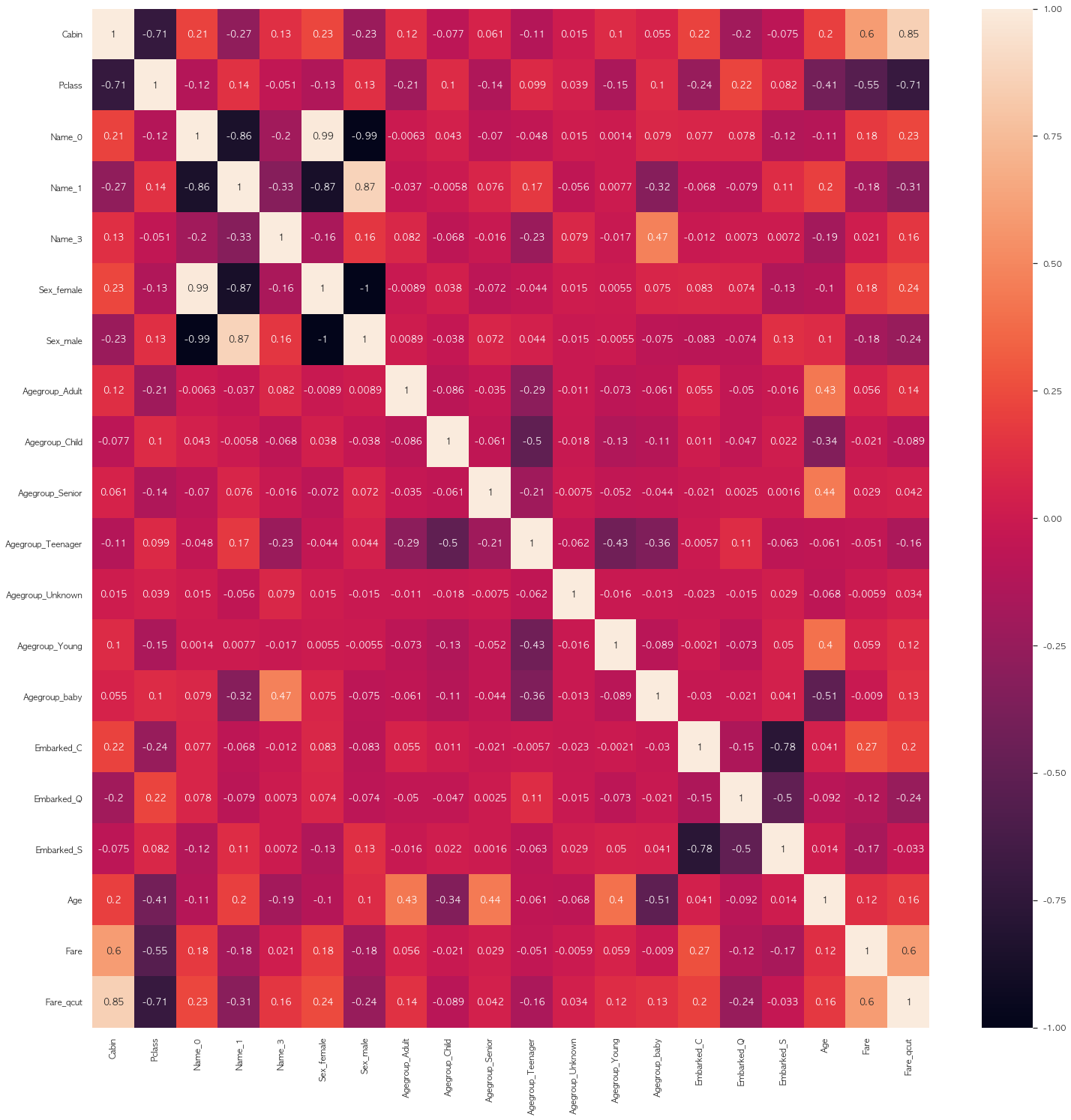
4. Model
4-1. Baseline
from sklearn import model_selection
from sklearn import ensemble, gaussian_process, linear_model, naive_bayes, neighbors, svm, tree, discriminant_analysis
from xgboost import XGBClassifier
# 베이스 모델
MODELS = [
# 앙상블 모델
ensemble.AdaBoostClassifier(),
ensemble.BaggingClassifier(),
ensemble.ExtraTreesClassifier(),
ensemble.GradientBoostingClassifier(),
ensemble.RandomForestClassifier(),
# 가우시안 모델
gaussian_process.GaussianProcessClassifier(),
# 선형 모델
linear_model.LogisticRegressionCV(),
linear_model.PassiveAggressiveClassifier(),
linear_model.RidgeClassifierCV(),
linear_model.SGDClassifier(),
linear_model.Perceptron(),
# 나이브베이지안 모델
naive_bayes.BernoulliNB(),
naive_bayes.GaussianNB(),
# 이웃기반 모델
neighbors.KNeighborsClassifier(),
# SVM
svm.SVC(probability = True),
svm.NuSVC(probability = True),
svm.LinearSVC(),
# 트리 모델
tree.DecisionTreeClassifier(),
tree.ExtraTreeClassifier(),
# 선형판별분석
discriminant_analysis.LinearDiscriminantAnalysis(),
discriminant_analysis.QuadraticDiscriminantAnalysis(),
# xgboost
XGBClassifier()
]
# cross validation
cv_split = model_selection.ShuffleSplit(n_splits = 10, test_size = 0.2, train_size = 0.8, random_state = 42 ) # run model 10x with 60/30 split intentionally leaving out 10%
# 모델 비교를 위한 데이터프레임 생성
Model_columns = ['Model Name', 'Model Parameters', 'Model Train Accuracy Mean', 'Model Test Accuracy Mean', 'Model Test Accuracy 3*STD' ,'Model Time']
Model_compare = pd.DataFrame(columns = Model_columns)# 모델별 predict 결과 저장
Model_predict = Y.copy()
# MLA_compare 데이터프레임에 각 모델 결과 저장
row_index = 0
for alg in MODELS:
# 모델별 base Parameter
Model_name = alg.__class__.__name__
Model_compare.loc[row_index, 'Model Name'] = Model_name
Model_compare.loc[row_index, 'Model Parameters'] = str(alg.get_params())
cv_results = model_selection.cross_validate(alg, X = X, y = Y, cv = cv_split, return_train_score = True)
Model_compare.loc[row_index, 'Model Time'] = cv_results['fit_time'].mean()
Model_compare.loc[row_index, 'Model Train Accuracy Mean'] = cv_results['train_score'].mean() # cross_validate에서 'train_score' 나오지 않음
Model_compare.loc[row_index, 'Model Test Accuracy Mean'] = cv_results['test_score'].mean()
Model_compare.loc[row_index, 'Model Test Accuracy 3*STD'] = cv_results['test_score'].std()*3
# 모델별 predict 값 저장
alg.fit(X, Y)
Model_predict[Model_name] = alg.predict(X)
row_index+=1Model_compare = Model_compare.sort_values('Model Test Accuracy Mean', ascending = False).reset_index(drop = True)
Model_compare| Model Name | Model Parameters | Model Train Accuracy Mean | Model Test Accuracy Mean | Model Test Accuracy 3*STD | Model Time | |
|---|---|---|---|---|---|---|
| 0 | GradientBoostingClassifier | {'ccp_alpha': 0.0, 'criterion': 'friedman_mse'... | 0.903652 | 0.830168 | 0.075772 | 0.0869468 |
| 1 | XGBClassifier | {'base_score': 0.5, 'booster': 'gbtree', 'cols... | 0.883567 | 0.828492 | 0.0674776 | 0.0911861 |
| 2 | RandomForestClassifier | {'bootstrap': True, 'ccp_alpha': 0.0, 'class_w... | 0.984551 | 0.818436 | 0.0835471 | 0.135578 |
| 3 | AdaBoostClassifier | {'algorithm': 'SAMME.R', 'base_estimator': Non... | 0.83427 | 0.815642 | 0.0782522 | 0.0718477 |
| 4 | BaggingClassifier | {'base_estimator': None, 'bootstrap': True, 'b... | 0.968118 | 0.808939 | 0.0895669 | 0.0257989 |
| 5 | RidgeClassifierCV | {'alphas': array([ 0.1, 1. , 10. ]), 'class_w... | 0.806039 | 0.807263 | 0.0845497 | 0.0103013 |
| 6 | ExtraTreesClassifier | {'bootstrap': False, 'ccp_alpha': 0.0, 'class_... | 0.984551 | 0.805028 | 0.0798336 | 0.114957 |
| 7 | LinearDiscriminantAnalysis | {'n_components': None, 'priors': None, 'shrink... | 0.807584 | 0.805028 | 0.0780545 | 0.00644715 |
| 8 | LogisticRegressionCV | {'Cs': 10, 'class_weight': None, 'cv': None, '... | 0.809831 | 0.803911 | 0.0801846 | 0.984159 |
| 9 | BernoulliNB | {'alpha': 1.0, 'binarize': 0.0, 'class_prior':... | 0.786376 | 0.793855 | 0.0819174 | 0.00365911 |
| 10 | NuSVC | {'break_ties': False, 'cache_size': 200, 'clas... | 0.795646 | 0.789385 | 0.104678 | 0.09748 |
| 11 | DecisionTreeClassifier | {'ccp_alpha': 0.0, 'class_weight': None, 'crit... | 0.984551 | 0.788268 | 0.0907043 | 0.00587251 |
| 12 | ExtraTreeClassifier | {'ccp_alpha': 0.0, 'class_weight': None, 'crit... | 0.984551 | 0.780447 | 0.071911 | 0.00419157 |
| 13 | GaussianNB | {'priors': None, 'var_smoothing': 1e-09} | 0.760393 | 0.758659 | 0.0741229 | 0.00369005 |
| 14 | LinearSVC | {'C': 1.0, 'class_weight': None, 'dual': True,... | 0.72809 | 0.741899 | 0.314066 | 0.0319866 |
| 15 | GaussianProcessClassifier | {'copy_X_train': True, 'kernel': None, 'max_it... | 0.956601 | 0.726816 | 0.11279 | 0.159213 |
| 16 | KNeighborsClassifier | {'algorithm': 'auto', 'leaf_size': 30, 'metric... | 0.805197 | 0.722905 | 0.0536313 | 0.00471177 |
| 17 | SGDClassifier | {'alpha': 0.0001, 'average': False, 'class_wei... | 0.699719 | 0.714525 | 0.0903941 | 0.00653226 |
| 18 | PassiveAggressiveClassifier | {'C': 1.0, 'average': False, 'class_weight': N... | 0.684129 | 0.672067 | 0.282446 | 0.00496163 |
| 19 | SVC | {'C': 1.0, 'break_ties': False, 'cache_size': ... | 0.682022 | 0.667598 | 0.0700109 | 0.0661206 |
| 20 | Perceptron | {'alpha': 0.0001, 'class_weight': None, 'early... | 0.65618 | 0.651955 | 0.40516 | 0.00473375 |
| 21 | QuadraticDiscriminantAnalysis | {'priors': None, 'reg_param': 0.0, 'store_cova... | 0.569101 | 0.556425 | 0.305672 | 0.0052588 |
sns.barplot(x = 'Model Test Accuracy Mean', y = 'Model Name', data = Model_compare, color = 'm')

plt.title('Machine Learning Algorithm Accuracy Score \n')
plt.xlabel('Accuracy Score (%)')
plt.ylabel('Algorithm')
plt.show()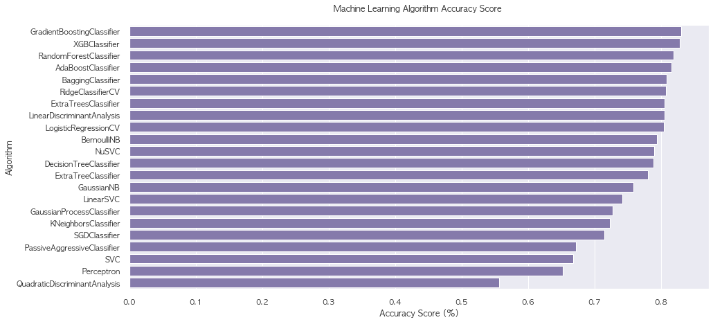
4-2. Ensemble
# 상위 10개 모델만 선정
TOP = []
for name in Model_compare['Model Name'].values:
    for alg in MODELS:
        if name in str(alg):
            try: # predict_proba 가 존재하는 모델만 선별
                alg.predict_proba
                v = (name, alg)
                TOP.append(v)
            except:
passTOP[('GradientBoostingClassifier', GradientBoostingClassifier()),
('XGBClassifier', XGBClassifier()),
('RandomForestClassifier', RandomForestClassifier()),
('AdaBoostClassifier', AdaBoostClassifier()),
('BaggingClassifier', BaggingClassifier()),
('ExtraTreesClassifier', ExtraTreesClassifier()),
('LinearDiscriminantAnalysis', LinearDiscriminantAnalysis()),
('LogisticRegressionCV', LogisticRegressionCV()),
('BernoulliNB', BernoulliNB()),
('NuSVC', NuSVC(probability=True)),
('DecisionTreeClassifier', DecisionTreeClassifier()),
('ExtraTreeClassifier', ExtraTreeClassifier()),
('GaussianNB', GaussianNB()),
('GaussianProcessClassifier', GaussianProcessClassifier()),
('KNeighborsClassifier', KNeighborsClassifier()),
('SVC', SVC(probability=True)),
('SVC', NuSVC(probability=True)),
('QuadraticDiscriminantAnalysis', QuadraticDiscriminantAnalysis())]vote_est = TOP[:9]vote_est[('GradientBoostingClassifier', GradientBoostingClassifier()),
('XGBClassifier', XGBClassifier()),
('RandomForestClassifier', RandomForestClassifier()),
('AdaBoostClassifier', AdaBoostClassifier()),
('BaggingClassifier', BaggingClassifier()),
('ExtraTreesClassifier', ExtraTreesClassifier()),
('LinearDiscriminantAnalysis', LinearDiscriminantAnalysis()),
('LogisticRegressionCV', LogisticRegressionCV()),
('BernoulliNB', BernoulliNB())]def voting(model_candidates):
N = len(model_candidates)
history = []
for i in reversed(range(2, N+1)):
vote_est = model_candidates[:i]
print('=' * 15, f'voting {i} Model', '=' * 15)
vote_hard = ensemble.VotingClassifier(estimators = vote_est , voting = 'hard')
vote_hard_cv = model_selection.cross_validate(vote_hard, X, Y, cv = cv_split)
# print("Hard Voting Test w/bin score mean: {:.2f}". format(vote_hard_cv['test_score'].mean()*100))
# print("Hard Voting Test w/bin score 3*std: +/- {:.2f}". format(vote_hard_cv['test_score'].std()*100*3))
print('-' * 40)
# Soft Vote
vote_soft = ensemble.VotingClassifier(estimators = vote_est , voting = 'soft')
vote_soft_cv = model_selection.cross_validate(vote_soft, X, Y, cv = cv_split)
# print("Soft Voting Test w/bin score mean: {:.2f}". format(vote_soft_cv['test_score'].mean()*100))
# print("Soft Voting Test w/bin score 3*std: +/- {:.2f}". format(vote_soft_cv['test_score'].std()*100*3))
value = [i, vote_hard_cv['test_score'].mean(), vote_soft_cv['test_score'].mean()]
history.append(value)
print('=' * 40)
return historyhistory = voting(vote_est)=============== voting 9 Model ===============
----------------------------------------
========================================
=============== voting 8 Model ===============
----------------------------------------
========================================
=============== voting 7 Model ===============
----------------------------------------
========================================
=============== voting 6 Model ===============
----------------------------------------
========================================
=============== voting 5 Model ===============
----------------------------------------
========================================
=============== voting 4 Model ===============
----------------------------------------
========================================
=============== voting 3 Model ===============
----------------------------------------
========================================
=============== voting 2 Model ===============
----------------------------------------
========================================pd.DataFrame(history, columns = ['model_cnt', 'hard_vote_score', 'soft_vote_score'])| model_cnt | hard_vote_score | soft_vote_score | |
|---|---|---|---|
| 0 | 9 | 0.836313 | 0.843017 |
| 1 | 8 | 0.836313 | 0.836872 |
| 2 | 7 | 0.837989 | 0.840782 |
| 3 | 6 | 0.829609 | 0.830168 |
| 4 | 5 | 0.834078 | 0.840782 |
| 5 | 4 | 0.829050 | 0.839106 |
| 6 | 3 | 0.835196 | 0.837430 |
| 7 | 2 | 0.831285 | 0.832961 |
4-3. HyperParameter Tuning
grid_n_estimator = [10, 50, 100, 300]
grid_ratio = [.1, .25, .5, .75, 1.0]
grid_learn = [.01, .03, .05, .1, .25]
grid_max_depth = [2, 4, 6, 8, 10, None]
grid_min_samples = [5, 10, .03, .05, .10]
grid_criterion = ['gini', 'entropy']
grid_bool = [True, False]
grid_seed = [0]

grid_params = {
                'RandomForestClassifier' : {
                    'n_estimators' : grid_n_estimator,
                    'criterion': grid_criterion,
                    'max_depth': grid_max_depth,
                    'oob_score': [True],
                    'random_state': grid_seed
                },

                'XGBClassifier' : {
                    'learning_rate': grid_learn,
                    'max_depth': [1,2,4,6,8,10],
                    'n_estimators': grid_n_estimator,
                    'seed': grid_seed
                },

                'GradientBoostingClassifier' : {
                    'learning_rate': [.05],
                    'n_estimators': [300],
                    'max_depth': grid_max_depth, #default=3
                    'random_state': grid_seed
                },

                'BaggingClassifier' : {
                    'n_estimators': grid_n_estimator,
                    'max_samples': grid_ratio,
                    'random_state': grid_seed
                },

                'LinearDiscriminantAnalysis' : {
                    'solver' : ['svd', 'lsqr', 'eigen']
                },

                'LogisticRegressionCV' : {
                    'fit_intercept': grid_bool,
                    'penalty': ['l1','l2'],
                    'solver': ['newton-cg', 'lbfgs', 'liblinear', 'sag', 'saga'],
                    'random_state': grid_seed
                },

                'AdaBoostClassifier' : {
                    'n_estimators': grid_n_estimator,
                    'learning_rate': grid_learn,
                    'random_state': grid_seed
                },

                'ExtraTreesClassifier' : {
                    'n_estimators': grid_n_estimator,
                    'criterion': grid_criterion,
                    'max_depth': grid_max_depth,
                    'random_state': grid_seed
                },

                'NuSVC' : {
                    'gamma': grid_ratio,
                    'decision_function_shape': ['ovo', 'ovr'],
                    'probability': [True],
                    'random_state': grid_seed
                }

}
import timevote_est[:6][('GradientBoostingClassifier', GradientBoostingClassifier()),
('XGBClassifier', XGBClassifier()),
('RandomForestClassifier', RandomForestClassifier()),
('AdaBoostClassifier', AdaBoostClassifier()),
('BaggingClassifier', BaggingClassifier()),
('ExtraTreesClassifier', ExtraTreesClassifier())]start_total = time.perf_counter()
i = int(input())
MODELS = vote_est[:i]
for name, model in MODELS:
start = time.perf_counter()
best_search = model_selection.GridSearchCV(estimator = model, param_grid = grid_params[name], cv = cv_split, scoring = 'roc_auc')
best_search.fit(X, Y)
run = time.perf_counter() - start
best_param = best_search.best_params_
print('The best parameter for {} is {} with a runtime of {:.2f} seconds.'.format(name, best_param, run))
model.set_params(**best_param)
run_total = time.perf_counter() - start_total
print('Total optimization time was {:.2f} minutes.'.format(run_total/60)) 6
The best parameter for GradientBoostingClassifier is {'learning_rate': 0.05, 'max_depth': 4, 'n_estimators': 300, 'random_state': 0} with a runtime of 54.52 seconds.
The best parameter for XGBClassifier is {'learning_rate': 0.03, 'max_depth': 4, 'n_estimators': 300, 'seed': 0} with a runtime of 159.25 seconds.
The best parameter for RandomForestClassifier is {'criterion': 'gini', 'max_depth': 8, 'n_estimators': 300, 'oob_score': True, 'random_state': 0} with a runtime of 88.92 seconds.
The best parameter for AdaBoostClassifier is {'learning_rate': 0.1, 'n_estimators': 300, 'random_state': 0} with a runtime of 33.23 seconds.
The best parameter for BaggingClassifier is {'max_samples': 0.25, 'n_estimators': 300, 'random_state': 0} with a runtime of 41.43 seconds.
The best parameter for ExtraTreesClassifier is {'criterion': 'gini', 'max_depth': 6, 'n_estimators': 300, 'random_state': 0} with a runtime of 57.15 seconds.
Total optimization time was 12.13 minutes.history = voting(vote_est)=============== voting 9 Model ===============
----------------------------------------
========================================
=============== voting 8 Model ===============
----------------------------------------
========================================
=============== voting 7 Model ===============
----------------------------------------
========================================
=============== voting 6 Model ===============
----------------------------------------
========================================
=============== voting 5 Model ===============
----------------------------------------
========================================
=============== voting 4 Model ===============
----------------------------------------
========================================
=============== voting 3 Model ===============
----------------------------------------
========================================
=============== voting 2 Model ===============
----------------------------------------
========================================pd.DataFrame(history, columns = ['model_cnt', 'hard_vote_score', 'soft_vote_score'])| model_cnt | hard_vote_score | soft_vote_score | |
|---|---|---|---|
| 0 | 9 | 0.827933 | 0.837430 |
| 1 | 8 | 0.836872 | 0.840782 |
| 2 | 7 | 0.838547 | 0.843017 |
| 3 | 6 | 0.843017 | 0.845251 |
| 4 | 5 | 0.844134 | 0.845810 |
| 5 | 4 | 0.839106 | 0.848045 |
| 6 | 3 | 0.848603 | 0.848045 |
| 7 | 2 | 0.844693 | 0.846927 |
i = 6
MODELS = vote_est[:i]

vote_hard = ensemble.VotingClassifier(estimators = MODELS , voting = 'hard')
vote_hard_cv = model_selection.cross_validate(vote_hard, X, Y, cv  = cv_split)
vote_hard.fit(X, Y)

print("Hard Voting Test w/bin score mean: {:.2f}". format(vote_hard_cv['test_score'].mean()*100))
print("Hard Voting Test w/bin score 3*std: +/- {:.2f}". format(vote_hard_cv['test_score'].std()*100*3))
print('-' * 40)

# Soft Vote
vote_soft = ensemble.VotingClassifier(estimators = MODELS , voting = 'soft')
vote_soft_cv = model_selection.cross_validate(vote_soft, X, Y, cv  = cv_split)
vote_soft.fit(X, Y)

print("Soft Voting Test w/bin score mean: {:.2f}". format(vote_soft_cv['test_score'].mean()*100))
print("Soft Voting Test w/bin score 3*std: +/- {:.2f}". format(vote_soft_cv['test_score'].std()*100*3))
print('=' * 40)
6
Hard Voting Test w/bin score mean: 84.30
Hard Voting Test w/bin score 3*std: +/- 6.89
----------------------------------------
Soft Voting Test w/bin score mean: 84.53
Soft Voting Test w/bin score 3*std: +/- 7.07
========================================5. submission
# test 전처리X_test, _ = preprocessing.transform(test)X_test.head()| Cabin | Pclass | Name_0 | Name_1 | Name_3 | Sex_female | Sex_male | Agegroup_Adult | Agegroup_Child | Agegroup_Senior | Agegroup_Teenager | Agegroup_Unknown | Agegroup_Young | Agegroup_baby | Embarked_C | Embarked_Q | Embarked_S | Age | Fare | Fare_qcut | |
|---|---|---|---|---|---|---|---|---|---|---|---|---|---|---|---|---|---|---|---|---|
| 0 | 1 | 3 | 0 | 1 | 0 | 0 | 1 | 0 | 0 | 0 | 1 | 0 | 0 | 0 | 0 | 1 | 0 | 34.5 | 7.8292 | 1.0 |
| 1 | 1 | 3 | 1 | 0 | 0 | 1 | 0 | 0 | 0 | 0 | 0 | 0 | 1 | 0 | 0 | 0 | 1 | 47.0 | 7.0000 | 0.0 |
| 2 | 1 | 2 | 0 | 1 | 0 | 0 | 1 | 0 | 0 | 1 | 0 | 0 | 0 | 0 | 0 | 1 | 0 | 62.0 | 9.6875 | 1.0 |
| 3 | 1 | 3 | 0 | 1 | 0 | 0 | 1 | 0 | 0 | 0 | 1 | 0 | 0 | 0 | 0 | 0 | 1 | 27.0 | 8.6625 | 1.0 |
| 4 | 2 | 3 | 1 | 0 | 0 | 1 | 0 | 0 | 0 | 0 | 1 | 0 | 0 | 0 | 0 | 0 | 1 | 22.0 | 12.2875 | 2.0 |
X_test.isnull().sum()Cabin 0
Pclass 0
Name_0 0
Name_1 0
Name_3 0
Sex_female 0
Sex_male 0
Agegroup_Adult 0
Agegroup_Child 0
Agegroup_Senior 0
Agegroup_Teenager 0
Agegroup_Unknown 0
Agegroup_Young 0
Agegroup_baby 0
Embarked_C 0
Embarked_Q 0
Embarked_S 0
Age 0
Fare 1
Fare_qcut 1
dtype: int64X_test = X_test.fillna(0)X.shape, X_test.shape((891, 20), (418, 20))5-1. prediction
sub = pd.read_csv(os.path.join('data', 'gender_submission.csv'))sub.head()| PassengerId | Survived | |
|---|---|---|
| 0 | 892 | 0 |
| 1 | 893 | 1 |
| 2 | 894 | 0 |
| 3 | 895 | 0 |
| 4 | 896 | 1 |
pred_vote_hard = vote_hard.predict(X_test)
pred_vote_soft = vote_soft.predict(X_test)
for md, pred in zip(['hard', 'soft'], [pred_vote_hard, pred_vote_soft]):
sub['Survived'] = pred
sub.to_csv(os.path.join('data', 'submission_{}.csv'.format(md)), index = False)