Dilation, linear-interpolation 그리고 Bilinear upsampling

현재 작성중인 PSPN(Pyramid Scene Parsing Network)논문 리뷰에 앞서, 함께 설명할 dilation, linear-interpolation 그리고 Bilinear upsampling에 대해서 간략하게 설명하고자 한다.

먼저 dilation에 대해서 설명하겠다.

Dilation (Dilated / Astrous Convolution)

PSPN을 구현하다 보면,

def get_backbone(layers):
    if layers == 50:
        weights = models.ResNet50_Weights.DEFAULT
        backbone = models.resnet50(
            weights=weights,
            replace_stride_with_dilation=[False, True, True]
        )
    elif layers == 101:
        weights = models.ResNet101_Weights.DEFAULT
        backbone = models.resnet101(
            weights=weights,
            replace_stride_with_dilation=[False, True, True]
        )

    backbone_layers = list(backbone.children())[:-2]
    backbone = nn.Sequential(*backbone_layers)

    return backbone

위와 같이 replace_stride_with_dilation=[False, True, True] 를 사용하게 된다.(위 코드는 PSPN에서 backbone으로 ResNet50을 불러오는 과정이다.)
이는 backbone모델로 줄어든 Feature Map이 위치 정보 손실을 야기하게 되어 사용하는 기법이다.

---

Dilation이란, feature map의 spatial 해상도를 줄이지 않고 Receptive Field만 키우기 위한 Convolution 기법이다.
Semantic Segmentation에서 사실상 필수적인 개념이다.

PSPN에서는 backbone 모델로 pre-trained된 ResNet50 혹은 ResNet101 모델을 사용한다.
일반적인 분류문제에서 ResNet을 거칠 때 Output Feature Map의 크기는 원본 이미지의 1/32 크기로 줄어든다.(*output stride=32)

PSPN에서 사용하는 입력 이미지 473x473의 크기는 $\frac{473}{8} \approx 59.1 \Rightarrow 60\times60$ 이 된다. (*output stride=8)

[이 때 output stride는 누적 stride를 말한다.]

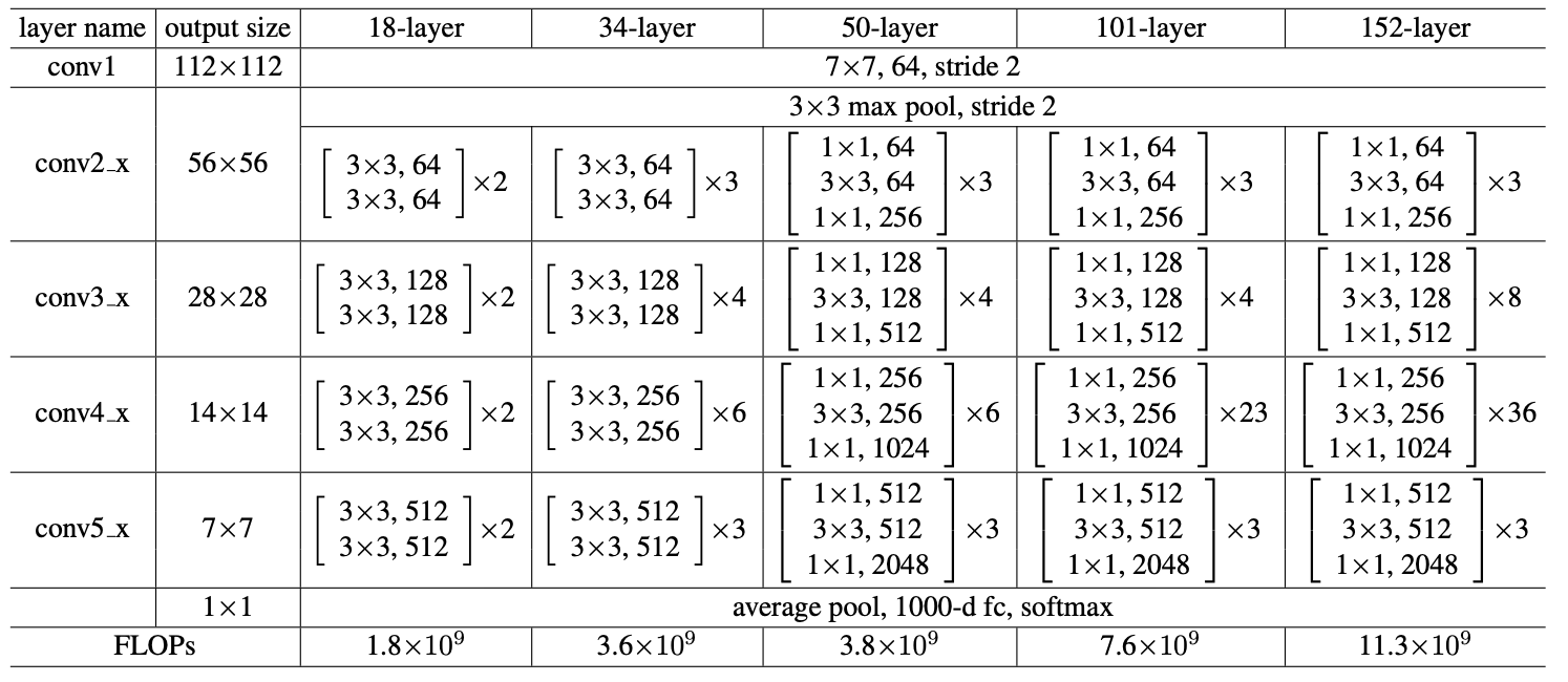
위 표는 ResNet 논문에서 가져온 Architecture 표이다.

잠시 구현한 ResNet의 코드 일부를 가져와서 살펴보자.

class ResNet18(nn.Module):
    def __init__(self, num_classes=1000):
        super().__init__()

        # in_channel 3 -> 64 변환 과정 (STEM) [conv1]
        self.conv1 = nn.Conv2d(3, 64, kernel_size=7, stride=2, padding=3, padding_mode='zeros')
        # 여기서 왜 bias를 왜 제거 해야할까?
        # BN이 Conv의 bias를 무력화하기 때문이다. -> BN의 Beta가 대신 역할 수행



        # 몇줄을 0padding으로 추가할지 output feature map 크기 구하는 공식 사용해서 직접 구하기
        self.bn = nn.BatchNorm2d(64)
        self.ReLU = nn.ReLU(inplace=True)
        self.maxPool = nn.MaxPool2d(kernel_size=3, stride=2, padding=1)

        self.layer1 = nn.Sequential(
            BasicBlock(64, 64, 1),
            BasicBlock(64, 64, 1)
        )
        self.layer2 = nn.Sequential(
            BasicBlock(64, 128, 2),
            BasicBlock(128, 128, 1)
        )
        self.layer3 = nn.Sequential(
            BasicBlock(128, 256, 2),
            BasicBlock(256, 256, 1)
        )
        self.layer4 = nn.Sequential(
            BasicBlock(256, 512, 2),
            BasicBlock(512, 512, 1)
        )

        # Head Designing..
        # GAP -> Flatten -> FC
        self.avgpool = nn.AdaptiveAvgPool2d((1, 1)) # 어떤 크기든 1x1로 압축
        self.fc = nn.Linear(512, num_classes)

위 코드와 ResNet논문의 표를 비교해서 살펴보자.

예제 코드	ResNet논문 표	크기(누적 stride)	dilation적용
INPUT	INPUT	473x473	원본
STEM (conv1+bn+ReLU +MaxPool2d)	conv1	119 x 119 (1/4)	초반엔 어쩔 수 없이 줄임
layer 1	conv2_$x$	119 x 119 (1/4)	원래 Stride가 1
layer 2	conv3_$x$	60 x 60 (1/8)	False
layer 3	conv4_$x$	60 x 60 (1/8)	True-여기서 False하면, 60보다 더 줄게됨. (Dilation:2)
layer 4	conv5_$x$	60 x 60 (1/8)	True (Dilation:4)

replace_stride_with_dilation 을 PSPN에서 사용한 코드를 보면(맨 처음), 실제 resnet50 클래스 안에

# 실제 라이브러리 내부 코드 (약간 단순화)
class ResNet(nn.Module):
    def __init__(self, block, layers, replace_stride_with_dilation, ...):
        
        # ... (중략) ...

        # ★ Layer 1: 얘는 리스트를 아예 안 봅니다. (항상 Stride=1이라 바꿀 게 없어서)
        self.layer1 = self._make_layer(block, 64, layers[0])

        # ★ Layer 2: 리스트의 첫 번째([0]) 값을 가져다 씀 -> False
        self.layer2 = self._make_layer(block, 128, layers[1], stride=2,
                                       dilate=replace_stride_with_dilation[0])

        # ★ Layer 3: 리스트의 두 번째([1]) 값을 가져다 씀 -> True
        self.layer3 = self._make_layer(block, 256, layers[2], stride=2,
                                       dilate=replace_stride_with_dilation[1])

        # ★ Layer 4: 리스트의 세 번째([2]) 값을 가져다 씀 -> True
        self.layer4 = self._make_layer(block, 512, layers[3], stride=2,
                                       dilate=replace_stride_with_dilation[2])

으로 하드코딩 되어있다.
때문에 replace_stride_with_dilation이 지정한 인덱스에 stride를 사용할지, dilation을 사용할지 결정할 수 있다.

이로써 Feature map의 크기를 60x60으로 유지할 수 있고, 위치정보 손실을 방지할 수 있게 된다.

Linear-Interpolation

Linear Interpolation (선형 보간)이란, 알려진 두 점 사이의 값을 그 직선 거리에 따라 선형적으로 추정하는 1차원 보간 방식이다.

두 점이 $(x_0, y_0), (x_1, y_1)$과 같이 주어졌을 때, 중간 지점 x에서의 값을
$y(x) = y_0 + \frac{x-x_0}{x_1 - x_0}(y_1-y_0)$으로 구할 수 있다.

두 점을 잇는 직선 위에서 값을 읽는 것이 핵심이다.

이것을 2D로 확장하면 Bilinear Interpolation이다.

Bilinear-Interpolation

Bilinear Interpolation은 가로(X)방향과 세로(Y)방향으로 Linear-Interpolation(선형 보간)을 두 번 적용한 것이다.

2차원 grid에서 주어지지 않은 좌표의 값을 추정할 때 사용한다.

어떠한 점 $P(x,y)$를 구하고자 할 때, 그 점을 둘러싼 4개의 가장 가까운 픽셀값을 사용하여 가중 평균을 구한다.

1. X축 방향으로 보간 : 위쪽 두 점 사이에서 한 번, 아래쪽 두 점 사이에서 한 번
2. Y축 방향으로 보간 : 위에서 구한 두 값을 사용하여 최종적으로 Y축 방향으로 보간하여 P를 찾는다.

위 1, 2번은 순서 상관없이 수행하면 된다.

PSPN을 구현할 때에는 입력이 (Batch, Channel, H, W)이기 때문에 mode='bilinear'를 사용하도록 한다.

구분	Linear Interpolation	Bilinear Interpolation
차원	1D (선 위에서의 보간)	2D (평면/이미지의 보간)
입력 텐서 형태	3D Tensor (N, C, L)	4D Tensor (N,C,H,W)
PyTorch	mode='linear'	mode='bilinear'
주요 용도	오디오 샘플링 속도 변환, 1D시계열 데이터 길이 변환	이미지 Resizing, Segmentation모델의 Upsampling

코드 비교

import torch 
import torch.nn.functional as F

#===== Linear Interpolation (1D 데이터용)======
input_1d = torch.tensor([[[10., 20.]]])
output_linear = F.interpolate(input_1d, scale_factor=2, mode='linear', align_corners=False)

print("Linear Interpolation")
print(f"\nInput : {input_1d.shape} -> {input_1d.tolist()}")
print(f"\nOutput : {output_linear.shape} -> {output_linear.tolist()}")


#===== Bilinear Interpolation (2D 이미지용) =======
input_2d = torch.tensor([[[[1., 2.],
	    					[3., 4.]]]])
ouptut_bilinear = F.interpolate(input_2d, scale_factor=2, mode='bilinear', align_corners=False)

print("\n\nBilinear Interpolation")
print(f"Input : {input_2d.shape}")
print(f"Output : {output_bilinear.shape}")