텍스트 마이닝 5가지 핵심 방법론 (w/python)

Euro·2025년 5월 30일

빈도분석

개념: 문서 집합에서 단어가 등장한 횟수(빈도)를 세어 가장 많이 쓰인 어휘를 파악한다.

수식:
단어 w의 단순 빈도

TF(w) = \sum_{d \in D} f_{d,w}

(여기서 $f_{d,w}$ 는 문서 $d$ 안의 단어 $w$ 등장 횟수)

개념 출처:https://nlp.stanford.edu/IR-book/pdf/irbookonlinereading.pdf

def get_top_counter(flat_list, count=100):
    return Counter(flat_list).most_common(count)

👉 가장 직관적인 지표지만, 전처리·가중치 없이는 노이즈에 취약함

TF-IDF

개념:

TF: 특정 문서에서 단어의 중요도
IDF: 코퍼스 전체에서 드문 단어에 더 높은 가중치
두 값을 곱해 문서 대비 전체 희소성까지 반영한 점수를 만든다.

수식:
단어 w, 문서 d, 전체 문서 수 $|\{\,d : w \in d\,\}|$

\mathrm{TF\!-\!IDF}(w,d)= TF_{w,d}\times \log\!\left(\frac{|D|}{|\{d:w\in d\}|}\right) \quad\text {}

출처: Spark Jones 1972

tfidf = TfidfVectorizer(
    tokenizer=lambda x: x,
    preprocessor=lambda x: x, 
    token_pattern=None  
) 

dtm = tfidf.fit_transform(joined_docs)
feature_names = tfidf.get_feature_names_out()

# 각 단어에 대한 TF-IDF의 합
tfidf_sum = dtm.sum(axis=0)  
word_count = pd.DataFrame({
    'word': feature_names,
    'tf-idf': tfidf_sum.A1  # 2D matrix → 1D array
})

# 상위 100개 추출
top_df = word_count.sort_values('tf-idf', ascending=False).head(100)

👉 TF-IDF는 ‘빈번 + 희소’를 동시에 고려해 핵심 키워드 추출

N-gram 분석

개념: 연속된 N개의 토큰을 하나의 단위로 보아 문맥·연어 패턴을 포착한다. (bi-gram, tri-gram …)

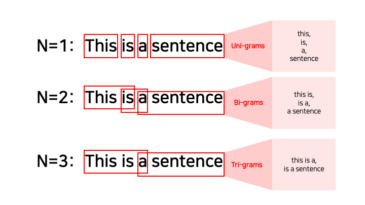
이미지 출처: Uni, Bi, Trigram("What is an N-gram", n.d.)

# PMI 계산 함수
def compute_pmi(bigram, unigram_counter, bigram_counter, total_len, total_bigrams):
    w1, w2 = bigram
    p_w1 = unigram_counter[w1] / total_len
    p_w2 = unigram_counter[w2] / total_len
    p_w1w2 = bigram_counter[bigram] / total_bigrams
    if p_w1 > 0 and p_w2 > 0 and p_w1w2 > 0:
        return log2(p_w1w2 / (p_w1 * p_w2))
    else:
        return 0

total_bigram_counter = Counter()
unigram_counter = Counter()

for tokens in tokenized_posts:
    unigram_counter.update(tokens)  # 단어 빈도
    finder = BigramCollocationFinder.from_words(tokens) # 바이그램 만듦 
    bigrams_freq = finder.ngram_fd.items()
    total_bigram_counter.update(dict(bigrams_freq))

# 전체 단어/바이그램 수
all_tokens = list(itertools.chain(*tokenized_posts))
total_len = len(all_tokens)
total_bigrams = sum(total_bigram_counter.values())

# 상위 100개 바이그램 기준으로 PMI 계산
top_100 = total_bigram_counter.most_common(100)

PMI(Pointsize Mutual Information): 두 확률 변수 사이의 상관성을 계량화하는 단위. (두 단어가 얼마나 자주 같이 등장하는지에 관한 정보를 수치화)

👉 서로 붙어 있는 연속 단어 묶음을 찾아냄으로써 문맥적인 통찰을 제공

Topic Modeling – LDA & BERTopic

1) LDA

개념: 주어진 문서에 대하여 각 문서에 어떤 주제들이 존재하는지에 대한 확률모형. 즉, 문서를 잠재 주제 분포 ( $\theta_d$ )와 주제-단어 분포 ( $\phi_k$ )의 곱으로 설명하는 생성 모델임.

수식:

p(\boldsymbol\theta,\mathbf z,\mathbf w \mid \alpha,\beta) \;=\; \prod_{d=1}^{M} \Bigl[ p(\theta_d \mid \alpha)\; \prod_{n=1}^{N_d} p(z_{d,n} \mid \theta_d)\; p(w_{d,n}\mid z_{d,n},\beta) \Bigr]

여기서

$M$ – 문서 수
$N_d$ – 문서 $d$ 의 단어 수
$\theta_d$ – 문서 $d$ 의 주제 분포
$z_{d,n}$ – $n$ 번째 단어의 주제 라벨
$w_{d,n}$ – 관측 단어
$\alpha,\beta$ – Dirichlet 하이퍼파라미터

출처: Blei, D. M., Ng, A. Y., & Jordan, M. I. “Latent Dirichlet Allocation.” JMLR, 3: 993-1022, 2003

동작과정 요약:

1. 문서마다 주제 분포 $\theta_d$ 를 Dirichlet 분포로부터 샘플링
1. 각 단어마다 주제를 선택하고 ( $z_{d,n} \sim \text{Multinomial}(\theta_d)$ )
1. 해당 주제에 맞는 단어를 샘플링 ( $w_{d,n} \sim \text{Multinomial}(\phi_{z_{d,n}})$ )

dictionary = corpora.Dictionary(total_tokens) 
dictionary.filter_extremes(no_below=10, no_above=0.5) # 너무 자주 나오거나, 희귀한 단어 제거
corpus = [dictionary.doc2bow(token) for token in total_tokens] 

# Coherence Score 
coherence_score=[]
top = 0
for i in range(2,10):
    model = gensim.models.ldamodel.LdaModel(corpus=corpus, id2word=dictionary, num_topics=i, passes= 5, random_state = 527)
    coherence_model = CoherenceModel(model, texts=total_tokens, dictionary=dictionary, coherence='c_v')
    coherence_lda = coherence_model.get_coherence()
    print('k=',i,'\nCoherence Score: ', coherence_lda)
    if i > 2 and coherence_score[top] < coherence_lda:
        print(top)
        top = i-2
    coherence_score.append(coherence_lda)
 
lda_model = gensim.models.ldamodel.LdaModel(corpus=corpus, id2word=dictionary , num_topics= top+2, passes= 5)
topics = lda_model.print_topics()

# 시각화 
prepared_data = gensimvis.prepare(lda_model, corpus , dictionary)  
pyLDAvis.display(prepared_data)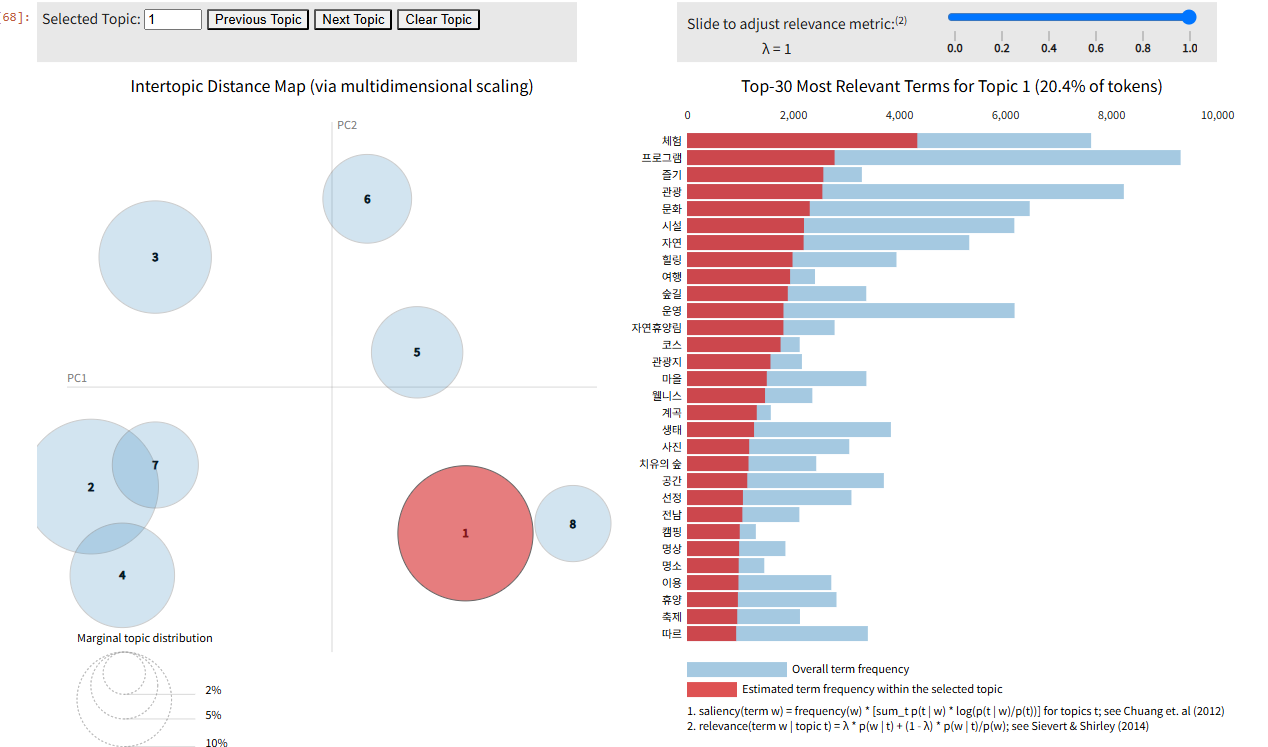

👉 단어 ↔ 주제 ↔ 문서의 삼각관계를 확률적으로 설명 가능

2) BERTopic

개념: BERT 임베딩과 군집화 알고리즘을 활용하여 텍스트 데이터에서 토픽을 추출하는 최신 방식

의미가 비슷한 문장을 벡터 공간에 모으고, 군집화한 뒤 그 안에서 핵심 단어를 뽑아 토픽을 구성

동작과정 요약:

1. Sentence-BERT 임베딩
1. HDBSCAN 클러스터링
1. 각 클러스터에 c-TF-IDF 로 대표 토픽 생성
- c-TF-IDF: 클러스터(=토픽) 단위의 문서 전체를 하나의 큰 문서처럼 간주하고, 각 토픽에서 중요한 단어를 추출하는 데 사용하는 변형된 TF-IDF 방식
- 일반 TF-IDF는 "문서 하나" 기준이지만, BERTopic은 "토픽(클러스터)"에 속한 다수의 문장을 하나의 큰 문서처럼 취급함

embedding_model = SentenceTransformer('../paraphrase-MiniLM-L6-v2')
vectorizer_model = TfidfVectorizer(tokenizer=lambda x: x.split(), token_pattern=None)

topic_model = BERTopic(
    embedding_model=embedding_model,
    vectorizer_model = vectorizer_model,
    top_n_words = 10,
    min_topic_size = 5,
    verbose = True
)

topics, probs = topic_model.fit_transform(docs)

rst = topic_model.get_topic_info()
for topic in range(len(rst)):
    print(rst.loc[topic, "Representation"])

👉 딥러닝 기반의 문장 의미 임베딩을 활용해 더 정교하고 문맥적인 토픽 분석 가능

항목	LDA	BERTopic
방식	확률 기반 생성 모델	임베딩 + 군집 기반
입력	단어 기반 문서 행렬	문장 임베딩 벡터
장점	해석이 수학적으로 명확함	문맥 이해, 짧은 문장에 강함
단점	문맥 반영 한계, 성능 민감	군집 품질에 따라 결과 편차 있음

CONCOR 분석

개념: CONvergence of iterated CORrelations –
동일한 유형의 객체들 간의 관계를 나타낸 행렬을 기반으로, 네트워크 구조상 유사한 위치나 기능을 하는 노드들을 찾아내는 군집화 기법이다.

상관분석을 반복 적용하여 점차 구조적 동등성에 수렴시키는 과정인 상관계수 반복 계산을 통해 구조적으로 동일한 역할(위치)을 가진 노드들을 찾아냄

동작과정 요약:
Python으로 생성

1. 공존 행렬 𝑀 선언

UCINET에서 실행

1. 열 z-score → 상관행렬 𝑅
1. 표준화·상관 반복 (수렴 시까지)
1. 최종 행렬 부호(±1)로 이진화 → 블록모델

UCINET 시각화 관련 내용은 https://chocolemon.tistory.com/154
여기에 잘 정리되어 있습니다!@

# 상위 100개 단어에 대한 공존 매트릭스 생성

top_n = 100
top_words = set([word for word, _ in word_freq.most_common(top_n)])

# 공존 관계 저장
co_occurrences = defaultdict(Counter)

# 상위 단어만 고려한 co-occurrence 계산
for tokens in tqdm(total_tokens):
    for i, word in enumerate(tokens):
        if word not in top_words:
            continue
        for j in range(max(0, i - window_size), min(len(tokens), i + window_size + 1)):
            if i != j and tokens[j] in top_words:
                co_occurrences[word][tokens[j]] += 1

# 단어 → 인덱스 매핑
selected_words = sorted(top_words)  # 정렬은 보기 편하게
word_index = {word: idx for idx, word in enumerate(selected_words)}

# 공존 행렬 초기화
co_matrix = np.zeros((len(selected_words), len(selected_words)), dtype=int)

# 값 채우기
for word, neighbors in co_occurrences.items():
    for neighbor, count in neighbors.items():
        i, j = word_index[word], word_index[neighbor]
        co_matrix[i][j] = count

# DataFrame 생성 및 저장
co_matrix_df = pd.DataFrame(co_matrix, index=selected_words, columns=selected_words)

#output 예시

[단어1]────┐
           ├──> [블록 A]
[단어2]────┘

[단어3]────┐
           ├──> [블록 B]
[단어4]────┘

→ 단어1과 단어2는 같은 단어들과 자주 같이 쓰이고, 단어3과 단어4는 또 다른 세트와 같이 쓰인다.
→ CONCOR는 이런 구조적 유사성을 찾아낸다.

👉반복 상관 → 수렴으로 네트워크 속 동등 그룹을 탐색

정말 간단하게 정리해봤는데, 수정/보완사항이 있으면 언제든지 피드백부탁드립니다 :)

Euro

이전 포스트

WBS(Work Breakdown Structure)

다음 포스트