yolov3 scratch를 해볼텐데, 저번 scratch 했던 것처럼 왜 이런 식으로 코딩을 했는지 생각하며 하나씩 하나씩 따라오는게 중요하다.
YoloV3 paper를 보면 architecture는 다음과 같다.
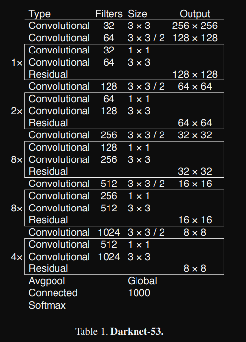
해당 architecture를 보면 잘 이해가 되지 않는데, 아래의 그림을 보고 좀더 이해하는 과정이 필요하다.
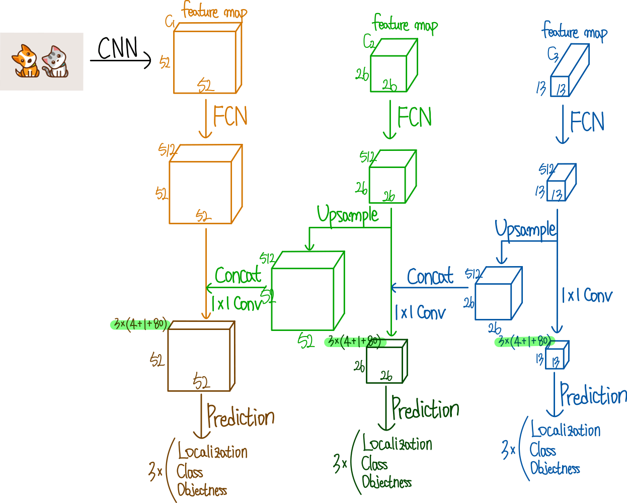
출처 : https://ffighting.net/deep-learning-paper-review/object-detection/yolo-v3/#google_vignette
어려운 구조는 아닌데, 다만 일반적인 CNN과 Residual만 있는 구조가 아니므로 추가적으로 생각할게 필요하다. tiny object까지 detection하기 위해서 upsample방식을 선택했고 이에 따라 성능을 향상 시켰다는 것이 중요하다.
YoloV3도 Yolov2에서 나온데로 Anchor형식이며 output도 Anchor 기준으로 shape를 구현하는데, 이는 모델을 구조를 보면서 추가적으로 설명하려고 한다.
우선 config부터 확인해보자.
# config
# (filter, kernel_size, stride)
config = [
    (32, 3, 1),
    (64, 3, 2),
    ["B", 1],
    (128, 3, 2),
    ["B", 2],
    (256, 3, 2),
    ["B", 8],
    (512, 3, 2),
    ["B", 8],
    (1024, 3, 2),
    ["B", 4],  # To this point is Darknet-53
    (512, 1, 1),
    (1024, 3, 1),
    "S",
    (256, 1, 1),
    "U",
    (256, 1, 1),
    (512, 3, 1),
    "S",
    (128, 1, 1),
    "U",
    (128, 1, 1),
    (256, 3, 1),
    "S",
]
전체 모델 구조는 다음과 같다. ["B", 4]아래 있는 (512, 1, 1), (1024, 3, 1)는 없어도 되긴하지만 모델의 성능을 향상시키기 위해 일부러 한층 더 깊은 신경만 구조를 추가했다.
B의 경우 Residual Block을 의미하고 1번 인덱스는 num_repeat로 반복 횟수를 의미한다.
S는 ScalePrediction인데, 우리가 예측하는 객체는 Anchor기준으로 예측이 된다. 따라서 Anchor크기에 따라 예측이 필요하다. Anchor의 크기는 [13, 26, 52]이며 이 scale에 따라 예측을 해야 하기 때문에 scale에 따른 예측 block이 필요하다.

Feature pyramid Network처럼 3개의 feature map을 뽑고 각각 총 3개의 Anchor로 예측을 하게 된다. 하나씩 만들어보자.
# model.py

import torch
from torch import nn

class CNNBlock(nn.Module):
	def __init__(self, in_channels, out_channels, bn_act=True, **kwargs):
    	super().__init__()

        self.bn_act = bn_act
        self.conv = nn.Conv2d(in_channels, out_channels, bias=False, **kwargs)
        self.bn = nn.BatchNorm2d(out_channels)
        self.act = nn.LeakyReLU(0.1)


    def forward(self, x):
    	if self.bn_act:
        	x = self.act(self.bn(self.conv(x)))

        else:
        	x = self.conv(x)

        return x
일반적인 CNNBlock이라 크게 어려운 것은 없으나 하나 다른건 있다. bn_act인데, 이는 나중에 ScalePrediction()을 구형하게 되는데, 해당 클래스는 최종 예측 단계이기 때문에 BatchNormalization이 수행되면 안되므로 조건문을 사용해야한다.
BatchNormalization은 Normalization이기 때문에 BatchNormalization의 input으로 들어가게 되면 일정한 분포로 정규화된다는 문제점이 생긴다. 마지막 예측 단계에서는 일정한 분포의 정규화가 필요하지 않고 설사 그것이 다른 쪽으로 편향되어 있더라도 모델에서 나오는 정확한 값이 필요하다. 따라서 BatchNormalization을 사용하지 않고 일반 CNN만 사용한다.
# model.py

class ResidualBlock(nn.Module):
	def __init__(self, in_channels, num_repeat, use_residual=True):
    	super().__init__()

        self.layers = nn.ModuleList()
        self.num_repeat = num_repeat
        self.use_residual = use_residual

        for _ in range(self.num_repeat):
        	self.layers += [
            	CNNBlock(in_channels, in_channels // 2, kernel_size=1, stride=1),
                CNNBlock(in_channels//2, in_channels, kernel_size=3, stride=1, padding=1)
            ]

    def forward(self, x):
    	for layers in self.layers:
        	if self.use_residual:
            	x = x + layers(x)

            else:
            	x = layers(x)

        return x
여기선 nn.ModuleList()를 사용한건데, nn.ModuleList()는 nn.Sequential()과 크게 다른 점은 foward()이다. 일반적으로 nn.Sequential()은 forward()가 자동적으로 실행되기 때문에, 제어를 할 수 없는 상태가 된다.
하지만 nn.ModuleList()는 그렇지 않기 때문에, 사용자가 직접 제어가 가능하게 된다. 극단적으로 예를 들자면
nn.Linear(4, 2) # 1
nn.Linear(2, 2) # 2
nn.Linear(2, 6) # 3
nn.ModuleList()로 해당 layer들을 append하게 되면 #2 -> #1 -> #3 순서로 실행시킬 수 있게된다. nn.Sequential()의 실행순서는 반드시 #1 -> #2 -> #3 순서대로 실행해야 하지만 nn.ModuleList()는 사용자가 유연하게 제어할 수 있다는 것이 장점이다.
# model.py

class ScalePrediction(nn.Module):
	def __init__(self, in_channels, num_classes, **kwargs):
    	super().__init__()

        self.layers = nn.ModuleList()

        self.layers += nn.Sequential(
        	[CNNBlock(in_channels, in_channels * 2, kernel_size=3, padding=1)],
            [CNNBlock(in_channels * 2, 3 * (num_classes + 5), bn_act=False, kernel_size=1)]
        )
        self.num_classes = num_classes

    def forward(self, x):
   		return (
        	self.layers(x).reshape(x.shape[0], 3, self.num_classes + 5, x.shape[2], x.shape[3])
            .permute(0, 1, 3, 4 ,2)
        )
위의 ResidualBlock도 그렇고 ScalePrediction도 보면 채널의 크기를 줄였다가 다시 복구 시키는 과정을 많이 거치는데, 이 과정은 모델에 꼭 필요한 요소이기도 하다. 채널을 줄이기만 하면 정보를 압축하는 역할을 계속 거치게 되는데, 이 과정이 지속되면 정보의 손실이 일어난다.
따라서 정보의 압축을 하면서 원래 크기로 복원하게 되면 노이즈와 중요도가 낮은 정보는 사라지고 필요한 정보는 유지될 가능성이 높아진다.
그 외에 여러가지가 있는데,
- 연산 비용이 절감된다.
- 비선형 표현이 강화된다.(LeakyReLU 같은 비선형 함수가 더 여러번 사용되므로)
- 네트워크 깊이 효과가 증가된다.
마지막 CNNBlock의 output을 보면 3 * (num_classes + 5)를 볼 수 있는데, 이는 prediction 과정이기 때문이다. 추후에 dataset에서 설명을 하겠지만 yolov3의 경우 [objectness, x, y, w, h, cls1, cls2, cls3...] 과 같이 이뤄져 있고 하나의 scale에 3개의 anchor가 예측하기 때문에 각 grid의 크기마다 3개의 공간만 만들면 된다.
예를들어, feature map의 크기가 1313, 2626, 5252의 총 3개의 scale에서 하나의 객체를 예측하는데, 총 9개의 Anchor box가 사용된다. 1313에서 3개, 2626에서 3개, 5252에서 3개를 사용하여 loss를 구하고 예측을 하게 된다.
이 과정에서는 grid scale 중 하나가 들어왔을때는(1313, 2626, 52*52중에서) 3개의 공간이 필요함므로(3개의 Anchor의 공간을 만들어줘야 하므로) 3개의 공간을 만들어준다.
self.layers(x).reshape(x.shape[0], 3, self.num_classes + 5, x.shape[2], x.shape[3]).permute(0, 1, 3, 4 ,2) 을 한 이유는 출력을 이와 같이 만들어줘야 tensor 계산이 편하기 때문.
class Yolov3(nn.Module):
	def __init__(self, in_channels=3, num_classes=80, **kwargs):
    	self.in_channels = in_channels
        self.num_classes = num_classes
        self.architecture = config
        self.module = self._create_block(self.architecture)

   	def forward(self, x):
    	output = []
        connection_up_r = []

        for layer in self.module:
        	if isinstance(layer, ScalePrediction):
            	output.append(layer(x))
            x = layer(x)

            if isinstance(layer, ResidualBlock) and layer.num_repeat == 8:
            	connection_up_r.append(x)

            elif isinstance(layer, Upsample):
            	x = torch.cat([x, connection_up_r[-1]], dim=1)
                connection_up_r.pop()


         return output


    def _create_block(self, config):
    	in_channels = self.in_channels
        layers = nn.ModuleList()

        for layer in config:
        	if isinstance(layer, tuple):
            	out_channels, kernel_size, stride= layer
                layers.append(
                	CNNBlock(in_channles, out_channels, kernel_size=kernel_size, padding=1 if kernel_size==3 else 0)
                )

        		in_channels = out_channels

            elif isinstance(layer, list):
            	num_repeat = layer[1]

                layers.append(
                	ResidualBlock(in_channels, num_repeat=num_repeat)
                )


        	elif isinstance(layer, str):
            	if layer == 'S':
                	layers += [
                    	ResidualBlock(in_channels, num_repeat=1, use_residual=False),
                        CNNBlock(in_channels, in_channels // 2, kernel_size=1),
                        ScalePrediction(in_channels // 2, num_classes= self.num_classes)
                    ]
                    in_channels = in_channels // 2

                else:
                	layers.append(nn.Upsample(scale_factor=2))
                    in_channels = in_channels * 3

          return layers
순서대로 이해하면 되는데, 추가적으로 설명할 부분은 바로 forward()이다.
def forward(self, x):
   	output = []
    connection_up_r = []

    for layer in self.module:
        if isinstance(layer, ScalePrediction):
            output.append(layer(x))
            x = layer(x)

        if isinstance(layer, ResidualBlock) and layer.num_repeat == 8:
            connection_up_r.append(x)

        elif isinstance(layer, Upsample):
            x = torch.cat([x, connection_up_r[-1]], dim=1)
            connection_up_r.pop()


     return output
output과 connection_up_r을 list 로 만든 이유는 다음과 같다.
output에는 총 9가지 정보가 담기는데, 이는 Scale에 따른 Anchor box 이므로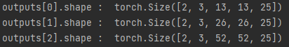
다음과 같은 shape를 갖는 tensor가 차곡차곡 저장된다.
connection_up_r의 경우에는 ResidualBlock이 num_repeat이 8이 될때의 shape이 차곡차곡 저장된다.
변수명이 다르긴한데, connection_up_r과 route_connections는 같은 역할을 한다.
이렇게 upsample된 정보 즉 high resolution과 low resolution을 합침으로써 high resoulution에서는 보지 못한 정보를 low resolution에서는 갖고 있므로 좀더 나은 성능을 발휘한다.