https://www.youtube.com/watch?v=Dt73QWZQck4&t=2213&ab_channel=DigitalSreeni
우선 다음 링크를 참고하는게 좋습니다. 설명도 친절하고 잘 되있습니다.
코드만 보실거면 이곳을 보시면 됩니다.
https://github.com/jw-chae/3d-Unet-medical-image-segmentation
환경은 다음과 같습니다.
nvcc(CUDA Compilation Tools): 11.5
CUDA: 12.2
python: 3.7
GPU:RTX3080
!pip install tensorflow==2.8.4
#%tensorflow_version 2.x
!pip install tensorflow==2.13.0
!pip install classification-models-3D
!pip install efficientnet-3D
!pip install segmentation-models-3D
!pip install patchify
여기서 분류 모델은 스스로 만들어서 사용해도 상관없습니다.
import tensorflow as tf
#import tensorflow.python.keras as keras
import keras
print(tf.__version__)
print(keras.__version__)

device_name = tf.test.gpu_device_name()
if device_name != '/device:GPU:0':
  raise SystemError('GPU device not found')
print('Found GPU at: {}'.format(device_name))
이제 환경설정이 잘 됐다면 GPU가 잡힐겁니다.
import segmentation_models_3D as sm그 다음 segmentation 모델을 입력하면 tf.keras framework를 사용한다고 나오면 성공입니다.
from skimage import io
from patchify import patchify, unpatchify
import numpy as np
from matplotlib import pyplot as plt
from tensorflow.keras import backend as K
from tensorflow.keras.utils import to_categorical
from sklearn.model_selection import train_test_split
import nibabel as nib
#Load input images and masks.
#Here we load 256x256x256 pixel volume. We will break it into patches of 64x64x64 for training.
patch_size = 64
stepsize=64
image_path = '/home/chae/segmentation/dataset/mr_train/mr_train_1001_image.nii.gz'
image_obj = nib.load(image_path)
image_data = image_obj.get_fdata()
print("imageshpae: ",image_data.shape)
img_patches = patchify(image_data, (patch_size,patch_size,patch_size), step=stepsize)  #Step=64 for 64 patches means no overlap
mask_path = '/home/chae/segmentation/dataset/mr_train/mr_train_1001_label.nii.gz'
mask_obj = nib.load(mask_path)
mask_data = mask_obj.get_fdata()
print("masksize: ",mask_data.shape)

mask_patches = patchify(mask_data, (patch_size,patch_size,patch_size), step=stepsize)
print("Number of patches:", img_patches.shape)
저같은 경우 CT,MRI 테스트 세트를 이용 하였고
이러한 의료영상 데이터는 보통 두가지 사용방법이 있습니다.
1.전체 이미지를 downsizing 해서 트레이닝
2.patch와 stepsize를 나누어서 트레이닝
3D영상은 예를들어 512x512x363의 이미지가 있다 가정하면
9500만개의 픽셀이 필요합니다.
흑백으로 하면 90MB가 필요하고
컬러로 하면 270 MB가 필요하며
이걸 그래픽카드가 버티지 못합니다.
그래서 보통 downzising이나 patch, stepsize를 나누는 방법을 사용하는데 downzising을 진행한다 해도
vram 80GB짜리 GPU 병렬구동 하는 수준이 아니면 사실상 못돌린다고 보면 됩니다.
patch_size 와 step_size
patch_size와 step_size는 이미지를 작은 부분(패치)으로 나누는 데 사용되는 중요한 매개변수입니다. 이들은 이미지 분할 및 패치 기반 학습에 널리 사용됩니다. 여기서의 주요 개념은 다음과 같습니다:
-
Patch Size (패치 크기): 이는 하나의 패치가 얼마나 큰지를 결정합니다.
예를 들어,patch_size = 64는 각 패치가 64x64x64 픽셀 크기를 가짐을 의미합니다.
이는 3D 이미지에서 각 패치가 64픽셀의 너비, 높이, 깊이를 가진다는 것을 의미합니다. -
Step Size (스텝 크기): 이는 연속적인 패치 사이의 간격을 결정합니다.
step_size = 64는 각 패치가 다음 패치와 64 픽셀만큼 떨어져 있음을 의미합니다.
이 경우, 패치 사이에 겹치는 부분이 없습니다.
만약step_size가patch_size보다 작다면, 패치들 사이에 겹치는 부분이 생기게 됩니다.
패치 기반 트레이닝 후에는, 학습된 모델을 사용하여 각각의 패치에 대한 예측을 수행하고, 이러한 예측들을 다시 조합하여 전체 이미지의 예측 결과를 복구할 수 있습니다.
이 과정은 unpatchify 함수를 사용하여 수행됩니다. 이 함수는 개별 패치들의 예측 결과를 원본 이미지의 크기로 재구성합니다.
예를 들어, 원본 이미지가 256x256x256 픽셀이고, patch_size가 64x64x64, step_size가 64라면, 원본 이미지는 64x64x64 크기의 64개의 패치로 나누어집니다.
각 패치에 대한 예측을 수행한 후, unpatchify 함수를 사용하여 이들을 다시 조합하면 원본 이미지의 크기인 256x256x256 픽셀의 예측 결과를 얻을 수 있습니다.
따라서, 패치 기반 트레이닝을 사용한 모델도 올바른 방법으로 패치를 재구성하면 전체 이미지 크기로 결과를 복구하는 것이 가능합니다.
근데 그럼 의문이 생깁니다.
363/64 는 정수가 아닌데?
어쩔 수 없습니다. 원본 이미지에 zero padding 진행해주셔야 합니다.
다운사이징을 진행하고 싶으시다면 다음과 같이 진행하시면 됩니다.
from scipy.ndimage import zoom

# 원본 이미지 데이터: image_data
# 다운사이징 비율
scale = 0.5  # 예시로 50% 축소

# 이미지 다운사이징
downsized_image_data = zoom(image_data, (scale, scale, scale))
downsized_mask_data = zoom(mask_data, (scale, scale, scale), order=0)

# 결과 확인
print("Original shape:", image_data.shape)
print("Downsized shape:", downsized_image_data.shape)
그 다음으로 다음 코드를 입력해서 재 구조화를 해줘야 합니다.
input_img = np.reshape(img_patches, (-1, img_patches.shape[3], img_patches.shape[4], img_patches.shape[5]))
input_mask = np.reshape(mask_patches, (-1, mask_patches.shape[3], mask_patches.shape[4], mask_patches.shape[5]))

print(input_img.shape)  # n_patches, x, y, z

print(img_patches.shape)
(128, 64, 64, 64)
(8, 8, 2, 64, 64, 64)
여기서 img_patches와 input_img의 차이는 차원의 구조와 데이터의 배열 방식에 있습니다. img_patches는 원본 이미지를 작은 패치로 나눈 것이고, input_img는 이러한 패치들을 신경망 모델에 입력하기 위해 재구조화한 것입니다.
-
img_patches의 형태 (Shape ofimg_patches):(8, 8, 2, 64, 64, 64)- 이 형태는 원본 이미지가 64x64x64 크기의 패치로 나누어진 것을 나타냅니다.
- 첫 번째 세 차원 (8, 8, 2)은 원본 이미지가 각각의 축(x, y, z)에 따라 몇 개의 패치로 나누어졌는지를 나타냅니다. 여기서는 x축으로 8개, y축으로 8개, z축으로 2개의 패치로 나누어졌습니다.
- 마지막 세 차원 (64, 64, 64)은 각 패치의 크기를 나타냅니다.
-
input_img의 형태 (Shape ofinput_img):(128, 64, 64, 64)- 이 형태는 신경망 모델에 입력하기 위해 패치들을 재구조화한 것입니다.
- 여기서 첫 번째 차원은 총 패치의 수를 나타냅니다. 원본 이미지가 8x8x2 = 128개의 패치로 나누어졌기 때문에 첫 번째 차원의 크기는 128입니다.
- 나머지 세 차원 (64, 64, 64)은 각 패치의 크기를 그대로 유지합니다.
재구조화 과정 (Reshaping Process):
np.reshape(img_patches, (-1, img_patches.shape[3], img_patches.shape[4], img_patches.shape[5]))- 여기서
-1은 NumPy가 자동으로 해당 차원의 크기를 계산하도록 지시합니다. 이 경우,-1은 모든 패치를 하나의 차원에 연속적으로 배열하라는 의미입니다. img_patches.shape[3], img_patches.shape[4], img_patches.shape[5]는 각 패치의 x, y, z 차원의 크기를 유지합니다.
따라서, input_img와 input_mask는 모델에 직접 입력할 수 있도록 패치들을 하나의 연속된 시퀀스로 재구조화한 것입니다.
이미지 라벨링
그 다음 과정은 이미지에 레이블을 찾는 것 입니다.
train_img = np.stack((input_img,)*3, axis=-1)
train_mask = np.expand_dims(input_mask, axis=4)
unique_values = np.unique(train_mask)
print(unique_values)
[ 0. 205. 420. 500. 550. 600. 820. 850.]
-
train_img = np.stack((input_img,)*3, axis=-1)input_img는 이미 처리된 이미지 데이터입니다. 의료영상 데이터는 보통 단일 채널 (예: 흑백 이미지)을 가지고 있습니다.np.stack((input_img,)*3, axis=-1)은input_img를 3번 복사하여 채널 차원을 확장합니다. 이는 일반적으로 RGB 이미지처럼 3채널 이미지를 요구하는 모델에 단일 채널 이미지를 사용할 때 필요합니다.- 결과적으로, 이 코드는 각 이미지의 채널 수를 1에서 3으로 확장합니다. 모든 3채널은 원본 단일 채널 이미지와 동일한 데이터를 가집니다.
-
train_mask = np.expand_dims(input_mask, axis=4)input_mask는 이미지의 레이블 또는 마스크 데이터입니다. 이 데이터도 보통 단일 채널을 가지고 있습니다.np.expand_dims(input_mask, axis=4)는 마스크 데이터에 새로운 차원을 추가합니다. 이는 일반적으로 모델이 예측해야 하는 출력 형식에 맞추기 위해 필요합니다.- 결과적으로, 이 코드는 마스크 데이터의 차원을 확장하여 모델의 출력 형식과 일치시킵니다.
-
unique_values = np.unique(train_mask)- 이 코드는
train_mask내의 고유한 값들을 찾습니다. np.unique함수는 배열 내의 모든 고유한 값을 찾아 정렬된 형태로 반환합니다.
- 이 코드는
저같은 경우엔 0,1,2,3... 이 아닌 0 205 420... 과 같은
특정 숫자로 나타났습니다.
이 레이블들을 재매핑 해보겠습니다.
def remap_label(label):

    label_mapping = {0:0 , 205: 1, 420: 2, 500: 3, 550: 4, 600: 5, 820: 6, 850: 7}
    return label_mapping.get(label, -1)  # 존재하지 않는 레이블은 -1로 처리

# train_mask의 모든 요소에 대해 remap_label 함수 적용
train_mask_remap = np.vectorize(remap_label)(train_mask)

# 새로운 레이블 값 확인
# -1 값을 제외하고 unique 값을 찾기
unique_values_remap = np.unique(train_mask_remap[train_mask_remap != -1])
print(unique_values_remap)
[0 1 2 3 4 5 6 7]
참고로 0은 배경입니다. 꼭 넣어주세요 안넣으면 segment자체가 안됩니다.
n_classes = 8

train_mask_cat = to_categorical(train_mask_remap, num_classes=n_classes)


X_train, X_test, y_train, y_test = train_test_split(train_img, train_mask_cat, test_size = 0.20, random_state = 0)
이제 이 이미지에 대한 train test split을 진행해줍니다.
한 장의 이미지로도 훈련은 가능합니다.
이제 loss 함수를 정의해봅시다.
loss 함수는 dice loss를 사용했습니다.
# Loss Function and coefficients to be used during training:
def dice_coefficient(y_true, y_pred):
    smoothing_factor = 1
    flat_y_true = K.flatten(y_true)
    flat_y_pred = K.flatten(y_pred)
    return (2. * K.sum(flat_y_true * flat_y_pred) + smoothing_factor) / (K.sum(flat_y_true) + K.sum(flat_y_pred) + smoothing_factor)

def dice_coefficient_loss(y_true, y_pred):
    return 1 - dice_coefficient(y_true, y_pred)
이제 모델을 정의하겠습니다.
#Define parameters for our model.

encoder_weights = 'imagenet'
BACKBONE = 'vgg16'  #Try vgg16, efficientnetb7, inceptionv3, resnet50
activation = 'softmax'
#patch_size = 64
channels=3
import tensorflow as tf

LR = 0.000001
optim = tf.keras.optimizers.Adam(LR)


# Segmentation models losses can be combined together by '+' and scaled by integer or float factor
# set class weights for dice_loss (car: 1.; pedestrian: 2.; background: 0.5;)
dice_loss = sm.losses.DiceLoss(class_weights=np.array([0.25,0.25, 0.25, 0.25,0.25, 0.25, 0.25, 0.25]))
focal_loss = sm.losses.CategoricalFocalLoss()
total_loss = dice_loss + (1 * focal_loss)

# actulally total_loss can be imported directly from library, above example just show you how to manipulate with losses
# total_loss = sm.losses.binary_focal_dice_loss # or sm.losses.categorical_focal_dice_loss

metrics = [sm.metrics.IOUScore(threshold=0.5), sm.metrics.FScore(threshold=0.5)]

preprocess_input = sm.get_preprocessing(BACKBONE)
backbone 모델로는 vgg16 resnet mobilenet등을 사용 가능합니다.
#Preprocess input data - otherwise you end up with garbage resutls
# and potentially model that does not converge.
X_train_prep = preprocess_input(X_train)
X_test_prep = preprocess_input(X_test)

print(f"X_train shape: {np.array(X_train).shape}")
print(f"y_train shape: {np.array(y_train).shape}")
print(f"X_test shape: {np.array(X_test).shape}")
print(f"y_test shape: {np.array(y_test).shape}")
X_train shape: (102, 64, 64, 64, 3)
y_train shape: (102, 64, 64, 64, 8)
X_test shape: (26, 64, 64, 64, 3)
y_test shape: (26, 64, 64, 64, 8)
이제 모델을 입력해줍니다.
#Define the model. Here we use Unet but we can also use other model architectures from the library.
model = sm.Unet(BACKBONE, classes=n_classes,
                input_shape=(patch_size, patch_size, patch_size, channels),
                encoder_weights=encoder_weights,
                activation=activation)

model.compile(optimizer = optim, loss=total_loss, metrics=metrics)
print(model.summary())
Model: "model"
__________________________________________________________________________________________________
Layer (type) Output Shape Param # Connected to
==================================================================================================
input_1 (InputLayer) [(None, 64, 64, 64, 0 []
3)]
block1_conv1 (Conv3D) (None, 64, 64, 64, 5248 ['input_1[0][0]']
64)
block1_conv2 (Conv3D) (None, 64, 64, 64, 110656 ['block1_conv1[0][0]']
64)
block1_pool (MaxPooling3D) (None, 32, 32, 32, 0 ['block1_conv2[0][0]']
64)
block2_conv1 (Conv3D) (None, 32, 32, 32, 221312 ['block1_pool[0][0]']
128)
block2_conv2 (Conv3D) (None, 32, 32, 32, 442496 ['block2_conv1[0][0]']
128)
block2_pool (MaxPooling3D) (None, 16, 16, 16, 0 ['block2_conv2[0][0]']
128)
...
Trainable params: 71,231,240
Non-trainable params: 4,032이제 훈련을 진행합니다.
#Fit the model
history=model.fit(X_train_prep,
          y_train,
          batch_size=1,
          epochs=100,
          verbose=1,
          validation_data=(X_test_prep, y_test))
훈련이 끝나면 loss와 IOU를 확인할 수 있습니다.
###
#plot the training and validation IoU and loss at each epoch
loss = history.history['loss']
val_loss = history.history['val_loss']
epochs = range(1, len(loss) + 1)
plt.plot(epochs, loss, 'y', label='Training loss')
plt.plot(epochs, val_loss, 'r', label='Validation loss')
plt.title('Training and validation loss')
plt.xlabel('Epochs')
plt.ylabel('Loss')
plt.legend()
plt.show()

acc = history.history['iou_score']
val_acc = history.history['val_iou_score']

plt.plot(epochs, acc, 'y', label='Training IOU')
plt.plot(epochs, val_acc, 'r', label='Validation IOU')
plt.title('Training and validation IOU')
plt.xlabel('Epochs')
plt.ylabel('IOU')
plt.legend()
plt.show()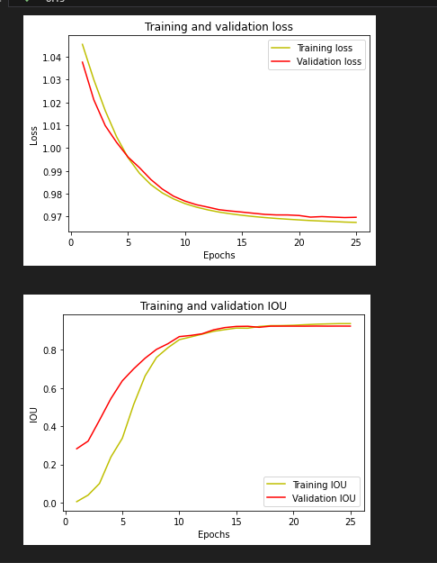
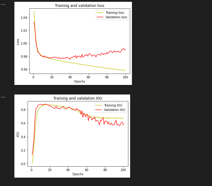
저같은 경우 train_loss val_loss iou는 다음과 같이 나왔습니다.
#Predict on the test data
from keras.models import load_model
my_model = load_model('/home/chae/segmentation/result/3D_mrmodel_vgg16_100epochs_2.h5', compile=False)
print(f'Type of my_model: {X_test_prep.shape}')
y_pred=my_model.predict(X_test_prep)
y_pred_argmax=np.argmax(y_pred, axis=4)
y_test_argmax = np.argmax(y_test, axis=4)

print(y_pred_argmax.shape)
print(y_test_argmax.shape)
print(np.unique(y_pred_argmax))
Type of my_model: (26, 64, 64, 64, 3)
(26, 64, 64, 64)
(26, 64, 64, 64)
[0 1 2 3 4 5 6 7]
이런식으로 y_pre_argmax의 unique_value가 잘 나오면 성공입니다.
# Using built in keras function for IoU
# Only works on TF > 2.0
from keras.metrics import MeanIoU
from keras.metrics import MeanIoU
n_classes = 8
IOU_keras = MeanIoU(num_classes=n_classes)
IOU_keras.update_state(y_test_argmax, y_pred_argmax)
print("Mean IoU =", IOU_keras.result().numpy())
Mean IoU = 0.122231014
mean IOU도 확인 해주시고요 , 저같은 경우 썩 좋은 결과는 아니였습니다.
유튜브 영상에선 잘 나왔는데 이유를 모르겠네요
이제 2D상에서 영상을 테스트 해봅시다.
결과확인
#Test some random images
import random
test_img_number = random.randint(0, len(X_test))
test_img = X_test[test_img_number]
ground_truth=y_test[test_img_number]
test_img_input=np.expand_dims(test_img, 0)
test_img_input1 = preprocess_input(test_img_input)
test_pred1 = my_model.predict(test_img_input1)
test_prediction1 = np.argmax(test_pred1, axis=4)[0,:,:,:]
print(test_prediction1.shape)
ground_truth_argmax = np.argmax(ground_truth, axis=3)
print(test_img.shape)
#Plot individual slices from test predictions for verification
slice = 31
slice1 = 31
slice2 = 31
plt.figure(figsize=(12, 8))
plt.subplot(231)
plt.title('Testing Image')
plt.imshow(test_img[slice1,:slice2,:,0], cmap='gray')
plt.subplot(232)
plt.title('Testing Label')
plt.imshow(ground_truth_argmax[slice,:slice2,:])
plt.subplot(233)
plt.title('Prediction on test image')
plt.imshow(test_prediction1[slice,:slice2,:])
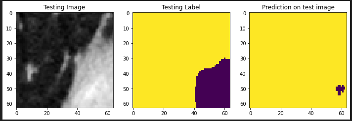
plt.show()
결과값
2D
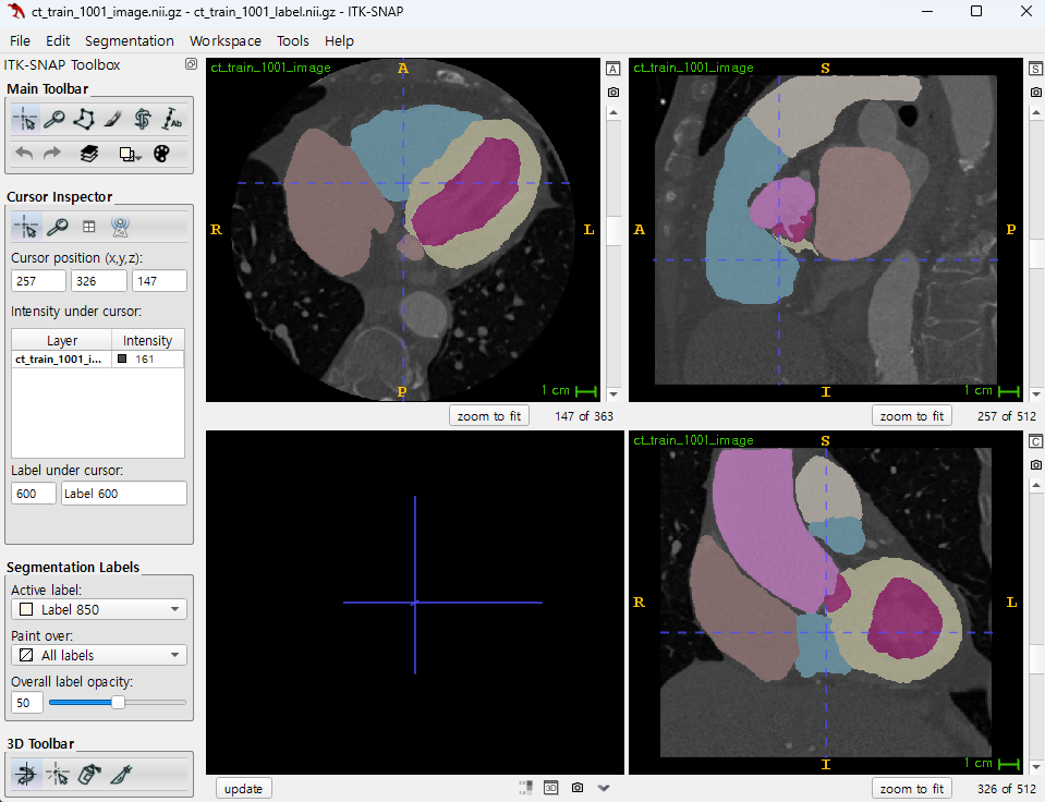
3D
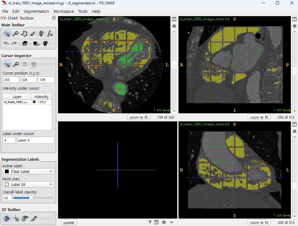
GT
망했네요 IOU 값으로는 상상도 안되는 나올 수 없는 수치가 나옵니다.
protein struct 때도 그렇고 데이터 전처리 난이도부터 해서 gpu가 성능이 아주 좋지 않으면 훈련자체가 불가능한 것 같습니다.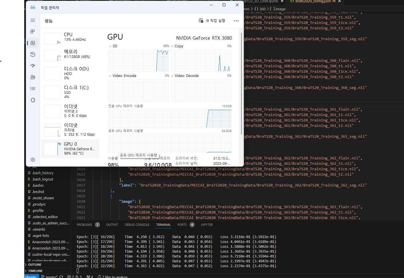
실패사례

다음은 실패사례들 입니다.
pytroch tensorflow는 파이썬, cuda, cudnn 버전 신경써야함
안맞으면 그래픽 카드 인식을 못해서 시작조차 못함
GPT가 시킨거 3번이상 안되면 직접 찾아보고 해결할 것
background label 없애는 멍청한 짓은 절대 하지 말것
이미지 사이즈 크면 죽음(patch size로 조절가능)
patch size 너무 작으면 죽음(batch 2000 나와서 그런가?)
output 네트워크 크기 안맞으면 죽음
lr 크면 죽음 (Nan)
네트워크 크기 크면 그래픽카드 죽음
훈련끝나고 그래픽카드 죽으면 그래픽카드 vram 죽이고 다시 시작해야함
val loss nan이면 훈련 안됨 다시 해야돼
개복치도 이런 개복치가 없네 진짜
기초 확실히 다지고 시작할 것
2D에 대한 이해도 제대로 못하고 3D로 넘어가는건 어불성설