There were a lot of improvement for this model.
Change in # of Features
The biggest change is that I added more columns for the dataset. It now refers to:
- RSI
- MACD
- Bollinger Bands
- ATR
- VIX_Relative
def get_dataset_columns(ticker, period="1y", window_size=60):
    df = yf.Tickers(ticker).history(period=period, progress=False)
    vix_data = yf.Tickers("^VIX").history(period=period, progress=False)

    if isinstance(df.columns, pd.MultiIndex):
        df.columns = df.columns.droplevel(1)
    if isinstance(vix_data.columns, pd.MultiIndex):
        vix_data.columns = vix_data.columns.droplevel(1)

    df = df.ffill().dropna()
    vix_data = vix_data.reindex(df.index).ffill()

    open_trend = apply_ssa_trend(df['Open'].values, window=int((window_size/4)))
    vix_trend  = apply_ssa_trend(vix_data['Open'].values, window=int((window_size/4)))

    min_len = min(len(df), len(open_trend), len(vix_trend))
    df = df.iloc[:min_len]

    ########################################################################

    # Features

    df['Open_Trend'] = open_trend[:min_len]
    df['Vix_Trend'] = vix_trend[:min_len]
    df['Trend_Diff'] = df['Open'] - df['Open_Trend']
    df['Vix_Trend_Diff'] = vix_data['Open'] - df['Vix_Trend']

    df['RSI'] = ta.rsi(df['Open'], length=14)

    macd = ta.macd(df['Open'])
    df = pd.concat([df, macd], axis=1)

    bbands = ta.bbands(df['Open'], length=20)
    df = pd.concat([df, bbands], axis=1)

    df['ATR'] = ta.atr(df['High'], df['Low'], df['Open'], length=14)

    df['VIX_Rel'] = vix_data['Open'] / vix_data['Open'].rolling(20).mean()

    ########################################################################

    # Target

    df['Target'] = (df['Open'].shift(-1) - df['Open']) / df['Open'] * 100
    # df['Target'] = np.log(df['Open'].shift(-1) / df['Open']) * 100
    # df['Target'] = df['Open'].shift(-1)

    ########################################################################

    df = df.iloc[:-1]

    df = df.drop(df.index[0])
    # df = df.drop(['High', 'Low', 'Volume', 'Close', 'Stock Splits', 'Dividends'], axis=1)

    df.columns.name = None
    exclude_cols = ['Open', 'High', 'Low', 'Close', 'Adj Close', 'Volume', 'Target']
    feature_cols = [c for c in df.columns if c not in exclude_cols]
    target_col = ["Target"]

    return df, feature_cols, target_col

def get_full_dataset(tickers, period="1y", window_size=60, test_size=0.2):
    X_total, y_total = [], []

    for ticker in tickers:
        df, feature_cols, target_col = get_dataset_columns(ticker, period=period, window_size=window_size)
        data_x = df[feature_cols].values
        data_y = df[target_col].values

        for i in range(len(df) - window_size):
            window_x = data_x[i : i + window_size]
            window_y = data_y[i + window_size]

            window_x = normalize_window(window_x)

            X_total.append(window_x)
            y_total.append(window_y)

    X_data = np.array(X_total)
    y_data = np.array(y_total)

    nan_mask = np.isnan(X_data).any(axis=(1, 2))
    X_data = X_data[~nan_mask]
    y_data = y_data[~nan_mask]

    print(f"NaN Deleted: {np.sum(nan_mask)}")

    test_first_index = int(len(X_data) * (1 - test_size))
    X_train, X_test = X_data[:test_first_index], X_data[test_first_index:]
    y_train, y_test = y_data[:test_first_index], y_data[test_first_index:]

    print("""
    X_train Shape : {}
    X_test Shape : {}
    y_train Shape : {}
    y_test Shape : {}
    """.format(X_train.shape, X_test.shape, y_train.shape, y_test.shape))

    return X_train, X_test, y_train, y_test
Same preprocessing steps can be performed for real life predictions
def get_data_for_prediction(ticker, period="120d", window_size=60):
    df, feature_cols, _ = get_dataset_columns(ticker, period=period, window=window_size)

    if len(df) < window_size:
        raise ValueError("Not enough rows")

    X = df[feature_cols].iloc[-window_size:].values

    if np.isnan(X).any():
        raise ValueError("NaN detected in prediction window")

    X = normalize_window(X)

    X = X.reshape(1, window_size, len(feature_cols))

    return X
The same CNN-LSTM model is used
def get_CNN_LSTM_hybrid(window_size=60, feature_num=3):
    dropout_rate = 0.2

    input_layer = Input(shape=(window_size, feature_num), name="Input")

    x = Conv1D(filters=64, kernel_size=3, strides=1, padding='same', activation='relu', name="Conv1D_1")(input_layer)
    x = LayerNormalization(name="LayerNormalization_1")(x)
    x = Conv1D(filters=64, kernel_size=3, strides=1, padding='same', activation='relu', name="Conv1D_2")(x)
    x = LayerNormalization(name="LayerNormalization_2")(x)

    x = MaxPooling1D(pool_size=2, name="Max_Pooling")(x)

    x = LSTM(64, return_sequences=True, name="LSTM_1")(x)
    x = Dropout(dropout_rate, name="Dropout_1")(x)
    x = BatchNormalization(name="BatchNormalization_1")(x)

    x = LSTM(32, return_sequences=False, name="LSTM_2")(x)
    x = Dropout(dropout_rate, name="Dropout_2")(x)
    x = BatchNormalization(name="BatchNormalization_2")(x)

    x = Dense(16, activation="relu", name="FullyConnected_1")(x)
    output_layer = Dense(1, activation="linear", name="Output")(x)

    model = Model(inputs=input_layer, outputs=output_layer, name='SSA_CNN_LSTM_Hybrid')

    optimizer = tf.keras.optimizers.Adam(learning_rate=0.001)
    model.compile(optimizer=optimizer,
                  loss='mse',
                  metrics=['mae', tf.keras.metrics.RootMeanSquaredError()])
    return model

CNN_LSTM_model = get_CNN_LSTM_hybrid(window_size, feature_num)
Evaluating
Unlike how I only evaluated the model by ‘rise’ and ‘fall’, now I added ‘neutral (hold)’.
def make_3class_label(y, threshold=0.05):
labels = np.zeros_like(y, dtype=int)
labels[y > threshold] = 2
labels[(y > 0) & (y <= threshold)] = 1
labels[y <= 0] = 0
return labels
predictions = CNN_LSTM_model.predict(X_test)
print(pd.DataFrame(predictions).describe())
# base_point = pd.DataFrame(predictions).mean().item()
base_point = 0
class_names = ['Fall', 'Neutral', 'Rise']
threshold = 0.1
y_test_class = make_3class_label(y_test, threshold)
predictions_class = make_3class_label(predictions, threshold)
unique, counts = np.unique(y_test_class, return_counts=True)
print("Test set class distribution:")
for u, c in zip(unique, counts):
print(f"Class {u}: {c} samples")
unique, counts = np.unique(predictions_class, return_counts=True)
print("\nPrediction set class distribution:")
for u, c in zip(unique, counts):
print(f"Class {u}: {c} samples")
plt.figure(figsize=(8, 6))
cm = confusion_matrix(y_test_class, predictions_class)
sns.heatmap(cm, annot=True, fmt='d', cmap='YlGnBu',
xticklabels=class_names,
yticklabels=class_names)
plt.title('Market Direction Confusion Matrix')
plt.xlabel('Predicted Label')
plt.ylabel('True Label')
plt.show()
print("\nClassification Report:")
print(classification_report(y_test_class, predictions_class, target_names=class_names))
y_test_flat = y_test.flatten()
preds_flat = predictions.flatten()
comparison_df = pd.DataFrame({
'Actual': y_test_flat,
'Predicted': preds_flat
})
chunk_size = 200
y_min_limit = -3.5
y_max_limit = 3.5
total_len = len(comparison_df)
num_plots = int(np.ceil(total_len / chunk_size))
fig, axes = plt.subplots(num_plots, 1, figsize=(15, 2.5 * num_plots), sharex=False)
if num_plots == 1:
axes = [axes]
for i in range(num_plots):
start = i * chunk_size
end = min((i + 1) * chunk_size, total_len)
subset = comparison_df.iloc[start:end]
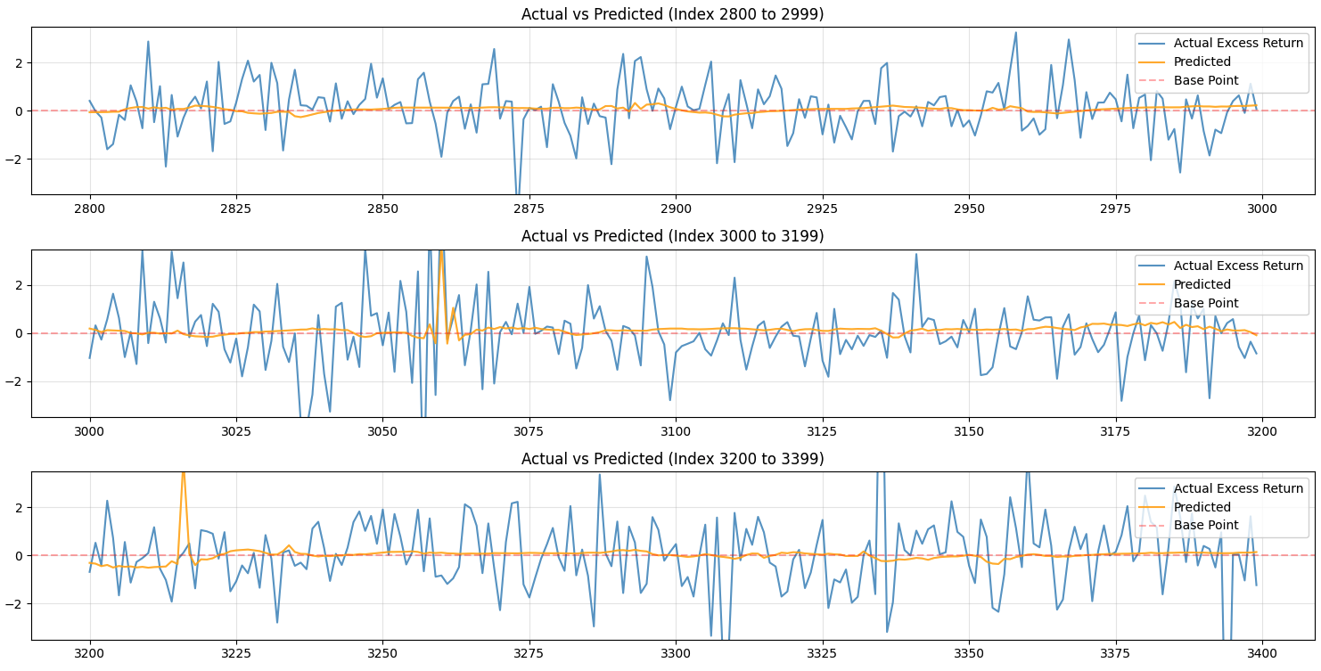
axes[i].plot(subset.index, subset['Actual'], label='Actual Excess Return', alpha=0.7)
axes[i].plot(subset.index, subset['Predicted'], label='Predicted', alpha=0.9, color='orange')
axes[i].set_ylim(y_min_limit, y_max_limit)
axes[i].axhline(base_point, label='Base Point', color='red', linestyle='--', alpha=0.3)
axes[i].set_title(f'Actual vs Predicted (Index {start} to {end-1})')
axes[i].legend(loc='upper right')
axes[i].grid(True, alpha=0.3)
plt.tight_layout()
plt.show()This is how my model is performing right now:
Test set class distribution:
Class 0: 3198 samples
Class 1: 240 samples
Class 2: 3142 samples

Prediction set class distribution:
Class 0: 2137 samples
Class 1: 1868 samples
Class 2: 2575 samples

Classification Report:
              precision    recall  f1-score   support

        Fall       0.49      0.32      0.39      3198
     Neutral       0.04      0.28      0.06       240
        Rise       0.47      0.38      0.42      3142

    accuracy                           0.35      6580
   macro avg       0.33      0.33      0.29      6580
weighted avg       0.46      0.35      0.39      6580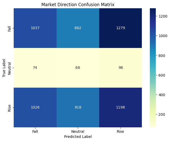
It is hard to say that my model is performing well, but it some times predict the return movement fairly well.
Backtesting
Next I implemented backtesting to evaluate the model in more detail.
def get_backtest_data(ticker, period="2y", window_size=60):
df, feature_cols, target_col = get_dataset_columns(ticker, period=period, window_size=window_size)
data_x = df[feature_cols].values
data_y = df[target_col].values
data_open_close = df[["Open", "Close"]].values
X_list = []
y_real = []
dates_list = []
actual_opens_list = []
for i in range(len(df) - window_size):
window_x = data_x[i : i + window_size]
window_y = data_y[i + window_size]
if np.isnan(window_x).any() or np.isnan(window_y).any():
continue
window_x = normalize_window(window_x)
current_open = data_open_close[i + window_size]
X_list.append(window_x)
y_real.append(window_y)
dates_list.append(df.index[i + window_size])
actual_opens_list.append(current_open)
return np.array(X_list), np.array(y_real), dates_list, feature_cols, np.array(actual_opens_list)
def backtest(model, ticker, period="1y", window_size=60, initial_capital=10000):
X_bt, y_bt, bt_dates, feature_cols, data_open = get_backtest_data(ticker, period=period, window_size=window_size)
predictions = model.predict(X_bt, verbose=0).flatten()
previous_signal = "INIT"
previous_correct_signal = "INIT"
cash = initial_capital
cash_when_not_traded = initial_capital
cash_fixed = 0
shares = 0
threshold = 0.1
portfolio_history = []
buy_count = 0
buy_correct_count = 0
actual_buy_count = 0
sell_count = 0
sell_correct_count = 0
actual_sell_count = 0
hold_count = 0
hold_correct_count = 0
actual_hold_count = 0
correct_pred_count = 0
wrong_pred_count = 0
current_open_price = data_open[0][0]
shares_when_not_traded = cash_when_not_traded // current_open_price
cash_when_not_traded -= shares_when_not_traded * current_open_price
for i in range(len(bt_dates)):
current_open_price = data_open[i][0]
y_act = y_bt[i][0]
cash_when_not_traded = shares_when_not_traded * current_open_price
if y_act >= threshold:
correct_signal = "BUY"
actual_buy_count += 1
elif y_act <= -0.5 * threshold:
correct_signal = "SELL"
actual_sell_count += 1
else:
correct_signal ="HOLD"
actual_hold_count += 1
correct = False
if predictions[i] >= threshold:
signal = "BUY"
buy_count += 1
if correct_signal == "BUY":
correct = True
elif predictions[i] <= -1 * threshold:
signal = "SELL"
sell_count += 1
if correct_signal == "SELL":
correct = True
else:
signal ="HOLD"
hold_count += 1
if correct_signal == "HOLD":
correct = True
action = "HOLD" if signal == previous_signal else signal
previous_signal = previous_signal if signal == "HOLD" else signal
if signal=="BUY" and cash > current_open_price:
share_num = cash // current_open_price
cash -= share_num * current_open_price
shares += share_num
elif signal=="SELL" and shares > 0:
cash += shares * current_open_price
shares = 0
if cash > initial_capital:
rev = cash - initial_capital
cash -= rev
cash_fixed += rev
total_value = cash_fixed + cash + (shares * current_open_price)
if correct:
correct_pred_count += 1
if signal == "BUY":
buy_correct_count += 1
elif signal == "SELL":
sell_correct_count += 1
elif signal == "HOLD":
hold_correct_count += 1
else :
wrong_pred_count += 1
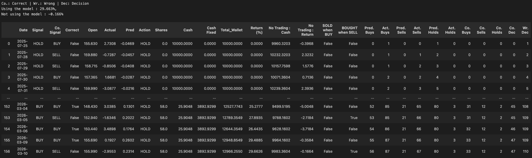
portfolio_history.append({
'Date': bt_dates[i],
'Signal': signal,
'Co. Signal': correct_signal,
'Correct': correct,
'Open': current_open_price,
'Actual': y_act,
'Pred': predictions[i],
'Action': action,
'Shares': shares,
'Cash': cash,
'Cash Fixed': cash_fixed,
'Total_Wallet': total_value,
'Return (%)': ((total_value - initial_capital) / initial_capital) * 100,
'No Trading : Cash': cash_when_not_traded,
'No Trading : Return': ((cash_when_not_traded - initial_capital) / initial_capital) * 100,
'SOLD when BUY':signal=="SELL" and correct_signal=="BUY",
'BOUGHT when SELL': signal=="BUY" and correct_signal=="SELL",
'Pred. Buys': buy_count,
'Act. Buys': actual_buy_count,
'Pred. Sells': sell_count,
'Act. Sells': actual_sell_count,
'Pred. Holds': hold_count,
'Act. Holds': actual_hold_count,
'Co. Buys': buy_correct_count,
'Co. Sells': sell_correct_count,
'Co. Holds': hold_correct_count,
'Co. Dec': correct_pred_count,
'Wr. Dec': wrong_pred_count,
})
result_df = pd.DataFrame(portfolio_history)
return result_df
def plotBacktestResult(df, print_detail=False):
row_num = 5 if print_detail else 2
figsize = (10, 12) if print_detail else (10, 6)
fig, axs = plt.subplots(row_num, 1, figsize=figsize, sharex=True)
other_cols = ["Shares", "Cash", "Cash Fixed"]
other_colors = ["#DC143C", "#9370DB", "#4169E1"]
buy_signals = df[df['Action'] == 'BUY']
sell_signals = df[df['Action'] == 'SELL']
axs[0].plot(df.index, df['Open'], label='Open', color='#4169E1', alpha=0.7)
axs[0].scatter(buy_signals.index, buy_signals['Open'],
marker='o', color='green', s=20, label='BOUGHT', edgecolor='black', zorder=5)
axs[0].scatter(sell_signals.index, sell_signals['Open'],
marker='o', color='red', s=20, label='SOLD', edgecolor='black', zorder=5)
axs[0].set_ylabel('Price (Open)')
axs[0].set_title('Open')
axs[0].legend(loc='upper left')
axs[1].plot(df.index, df['Return (%)'], label='Return using the model', color='#FFA500', alpha=0.7)
axs[1].plot(df.index, df['No Trading : Return'], label='Return if not traded', color='#2E8B57', alpha=0.7)
axs[1].axhline(y=0, color='gray', linestyle='--', linewidth=1.5)
axs[1].set_ylabel('Return %')
axs[1].set_title('Return Using This Model vs Not Trading')
axs[1].legend(loc='upper left')
if (print_detail):
for i, col_name in enumerate(other_cols):
ax_idx = i + 2
axs[ax_idx].plot(df.index, df[col_name], label=col_name, color=other_colors[i])
axs[ax_idx].set_title(col_name)
axs[ax_idx].legend(loc='upper left')
for ax in axs:
ax.grid(True, alpha=0.3)
plt.tight_layout()
plt.show()I used about 68 more companies to evaluate the model.
When I tested the model with Arista Networks Inc, the model resulted in a smaller return value than not buying anything.
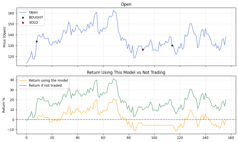
This is how the full result look like.
However, when I tested with Palantir, it resulted in a higher return.
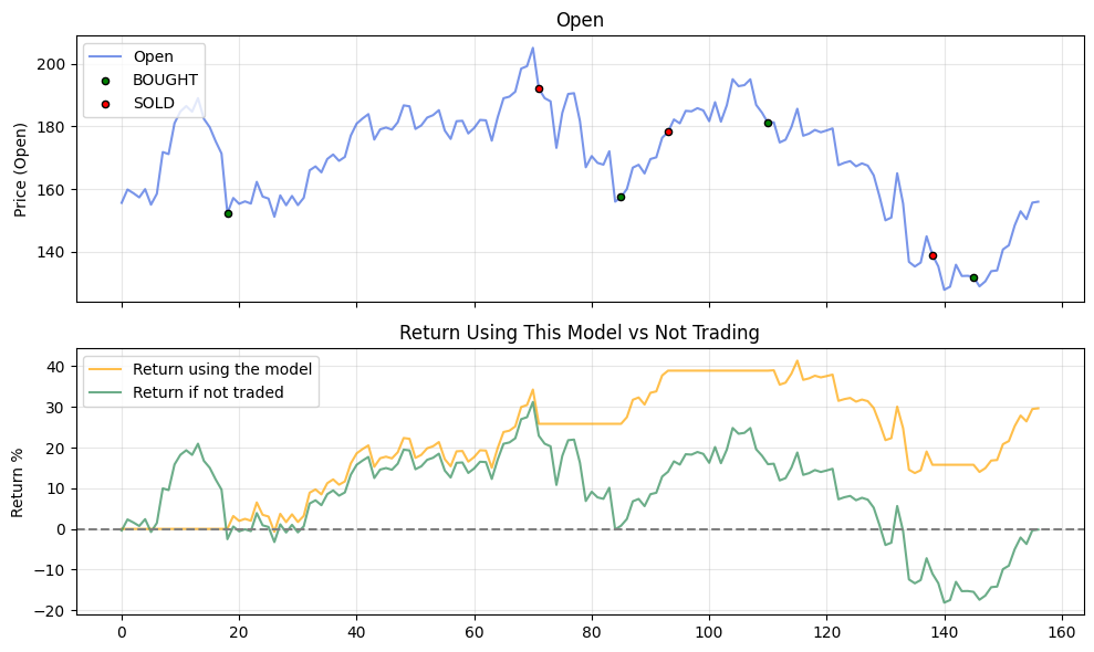
From these results, I found out that the model’s performance relies more on the actual movement of the stock price rather than its choices.
When testing with all 68 companies, the model performed better than the buy-and-hold strategy only 35 of the time.
Future Improvements
- Finding a better trading strategy is essential, as I believe that it will provide a better insight for my model’s performance.