Lec-05 1, 2 Logistic Classification

: 분류기법 중 하나로, 서로 다른 도형을 분류하는데 사용된다.

1. Logistic Regression

1) Classification

• Boundary Classification => 0과 1로 분류되는 것.
• ex) Pass/Fail, Spam/Not Spam, Real/Fake 등
• 학습 데이터

x_train = [[1, 2], [2, 3], [3, 1], [4, 3], [5, 3], [6, 2]]
y_train = [[0], [0], [0], [1], [1], [1]]  # binary labels

2) Logistic vs Linear

(데이터의 관점에서)

• Logistic : 2개의 케이스로 구분되고, 셀 수 있으며, 흩어져 있다. => 데이터가 구분된다.
• Linear : 데이터들이 연속적이다. 즉, 새로운 데이터가 들어와도 이어지는 값을 예측할 수 있다. => 데이터가 연속적이다.
• ex)

Logistic_Y = [[0], [0], [0], [1], [1], [1]]  # binary labels
Linear_Y  = [828.659973, 833.450012, 819.23999, 828.349976, 831.659973]  #   numeric

2. How to solve?

1) Hypothesis Representation

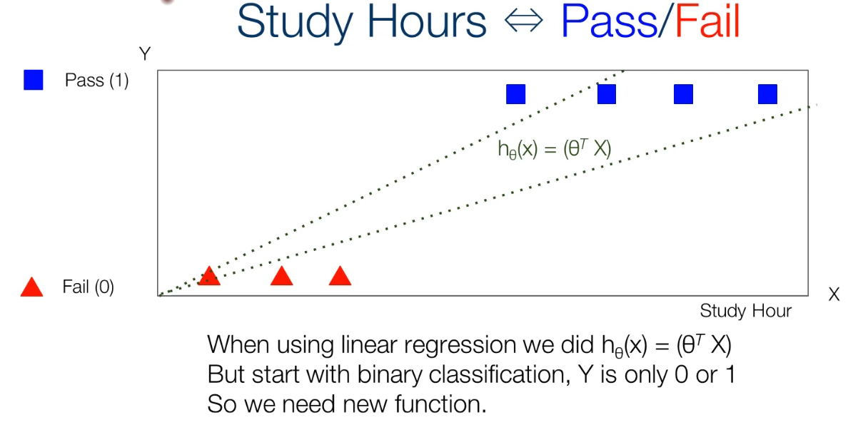
• 예제 : 공부 시간에 대한 Pass/Fail
• 기존 선형 회귀의 경우, $h_\theta(x) = \theta^T X$ 로 표현되는데, 이는 단순히 선으로만 나올 뿐, Pass와 Fail을 구분지어주지 못한다.
• => 그래프를 보면, 단순히 공부 시간에 따른 합격율만 계산할 수 있을 뿐, Pass와 Fail을 알 수 없다.

# Tensorflow Code
hypothesis = tf.matmul(X, θ) + b  # linear; θ is parameters

2) Sigmoid/Logistic Function

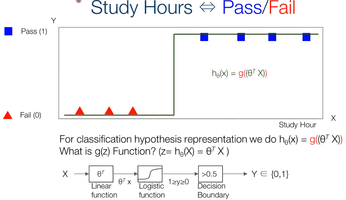
• 선형 회귀로는 분류를 할 수 없으므로, 새로운 수식이 필요하게 된다.
• => $h_\theta(X) = g(\theta^T X)$
• => 즉, 기존 $X$를 넣었을 때 $\theta$(= $W$)를 곱해서 나온 선형 값 $z$를 Logistic 함수로 $0$과 $1$ 구간으로 표현한다. 이를 임계값으로 0/1로 출력.
• $X \Rightarrow \theta^T X\,(Linear)\Rightarrow g(z)\,(Logistic)\Rightarrow 0 \le y \le 1 \Rightarrow greater\ than\ 0.5\,(Decision\ Boundary) \Rightarrow Y \in \{0,1\}$
• Logistic Function 정의: $g(z)=\dfrac{e^{z}}{e^{z}+1}=\dfrac{1}{1+e^{-z}}$
  • $z\to +\infty$이면 $g(z)\to 1$
  • $z\to -\infty$이면 $g(z)\to 0$

# Tensorflow Code
hypothesis = tf.sigmoid(z)          # z = tf.matmul(X, θ) + b
hypothesis = tf.div(1., 1. + tf.exp(z))

3) Decision Boundary (판정 규칙)

• 시그모이드: $g(z)=\dfrac{1}{1+e^{-z}}$. $0 \le y \le 1$ 범위.
• 판정 규칙: $g(z) > 0.5$ 이면 $y=1$, 아니면 $y=0$.
• 선형 경계: $h_\theta(x)=g(\theta_0+\theta_1 x_1+\theta_2 x_2)$ → 직선 경계. $x_1+x_2=0$가 판정 규칙 예시.
• 비선형 경계: $h_\theta(x)=g(\theta_0+\theta_1 x_1+\theta_3 x_1^2+\theta_4 x_2^2)$ → 곡선 경계. $x_1^2+x_2^2=1$
• 코드 판정

predicted = tf.cast(hypothesis > 0.5, dtype=tf.int32)

4) Cost Function

• 처음 랜덤하게 생성된 $\theta$(= weight)를 최적의 값으로 조정하는 것
• $h_\theta(X)=y$ 라는 것은, cost가 0이라는 것
• => $\text{cost}(h_\theta(X), y)=-y\log(h_\theta(X))-(1-y)\log(1-h_\theta(X))$

# Tensorflow Code
def loss_fn(hypothesis, labels):
    cost = -tf.reduce_mean(labels * tf.math.log(hypothesis) + (1 - labels) * tf.math.log(1 - hypothesis))
    return cost

• $J(\theta)=\dfrac{1}{m}\sum_{i=1}^{m}\dfrac{1}{2}\big(h_\theta(x^{(i)})-y^{(i)}\big)^2$
  • => 우리가 원하는 $J(\theta)$를 최소화하려면 $h_\theta(x^{(i)})$와 $y^{(i)}$의 차이가 0에 가까워야 한다.
  • => Logistic Regression에서는 $h_\theta(x)$가 $0\sim 1$의 실수형 확률값이 된다.
  • => 원하는 값은 0과 1의 이산값이므로, 단순 차이 제곱은 비불룩해질 수 있다.
  • => log를 쓰면 다음처럼 분해된다.

    Cost(hθ(x), y) = {
      -log(hθ(x))        if y = 1
      -log(1 - hθ(x))    if y = 0
    }

• 결합식: $\text{cost}(h_\theta(x),y)=-y\log(h_\theta(x))-(1-y)\log(1-h_\theta(x))$
  • => $y=1$일 때 $h_\theta(x)\to 1$이면 cost→0, $y=0$일 때 $h_\theta(x)\to 0$이면 cost→0.
  • => 두 식을 합치면 불룩한(convex) 형태가 된다.

# Tensorflow Code
cost = -tf.reduce_mean(labels * tf.log(hypothesis) + (1 - labels) * tf.log(1 - hypothesis))

5) Optimizer (Gradient Descent)

• 이렇게 구해진 Cost 함수
• $\text{cost}(h_\theta(x),y)=-y\log(h_\theta(x))-(1-y)\log(1-h_\theta(x))$
• Repeat { $\theta_j := \theta_j - \alpha \,\partial J/\partial \theta_j$ }
  • => 경사(미분값)로 최적값을 구한다.

# Tensorflow Code
def loss_fn_from_XY(X, y):
    z = tf.matmul(X, W) + b
    p = tf.math.sigmoid(z)
    return -tf.reduce_mean(y*tf.math.log(p) + (1-y)*tf.math.log(1-p))

def grad(X, y):
    with tf.GradientTape() as tape:
        loss_value = loss_fn_from_XY(X, y)
    return tape.gradient(loss_value, [W, b])

optimizer = tf.keras.optimizers.SGD(learning_rate=0.01)
grads = grad(X, y)
optimizer.apply_gradients(zip(grads, [W, b]))

6) Codes (Eager Execution)

• 학습 데이터

x_train = [
    [1., 2.],
    [2., 3.],
    [3., 1.],
    [4., 3.],
    [5., 3.],
    [6., 2.]
]
y_train = [
    [0.],
    [0.],
    [0.],
    [1.],
    [1.],
    [1.]
]
x_test = [[5., 2.]]
y_test = [[1.]]

• 전체 코드

import tensorflow as tf

dataset = tf.data.Dataset.from_tensor_slices((x_train, y_train)).batch(len(x_train))
W = tf.Variable(tf.zeros([2, 1]), name='weight')
b = tf.Variable(tf.zeros([1]), name='bias')
optimizer = tf.keras.optimizers.SGD(learning_rate=0.01)  <<- TF1 옵티마이저 교체

def logistic_regression(features):
    z = tf.matmul(features, W) + b
    return tf.math.sigmoid(z)  # 1/(1+exp(-z))  <<- tf.div/exp(z) 패턴 제거

def loss_fn(features, labels):
    p = logistic_regression(features)
    return -tf.reduce_mean(labels*tf.math.log(p) + (1-labels)*tf.math.log(1-p))  <<- tf.log → tf.math.log

def grad(features, labels):
    with tf.GradientTape() as tape:
        loss_value = loss_fn(features, labels)
    return tape.gradient(loss_value, [W, b])

EPOCHS = 1000
for step in range(EPOCHS):
    for features, labels in dataset:
        grads = grad(features, labels)
        optimizer.apply_gradients(zip(grads, [W, b]))
    if step % 100 == 0:
        print("Iter: {}, Loss: {:.4f}".format(step, loss_fn(features, labels).numpy()))

def accuracy_fn(hypothesis, labels):
    predicted = tf.cast(hypothesis > 0.5, dtype=tf.float32)
    accuracy = tf.reduce_mean(tf.cast(tf.equal(predicted, labels), dtype=tf.float32))
    return accuracy

test_acc = accuracy_fn(logistic_regression(x_test), y_test)

Summary

• Regression: 데이터를 가장 잘 대변하는 직선을 찾는 문제. 가설 $H(x)=Wx+b$, 비용 $\text{cost}(W,b)=\frac{1}{m}\sum_{i=1}^{m}(H(x_i)-y_i)^2$, 목표는 cost 최소화.
• Gradient Descent: 임의 초기값에서 시작해 기울기 방향으로 $W,b$를 반복 업데이트하여 최소점 탐색.
• Multi variable Linear Regression: 특징이 여러 개인 경우 $H(x_1,x_2,x_3,\dots)=w_1x_1+w_2x_2+\cdots+w_nx_n+b$. 행렬로 $H(X)=XW(+b)$로 표현.
• Logistic Regression: 분류. 선형 결합 $z=W^\top X+b$를 시그모이드 $g(z)=\frac{1}{1+e^{-z}}$에 넣어 $0\le y\le1$ 확률을 얻고 임계값(예: 0.5)으로 이진 결정.
• 로지스틱 비용 함수: $\text{cost}(h(x),y)=-\,y\log h(x)-(1-y)\log(1-h(x))$. 평균 비용 $J=\frac{1}{m}\sum \text{cost}$.
• 학습(최적화): 경사하강으로 $W,b$ 업데이트.

출처: 모두를 위한 딥러닝 강좌 2
https://www.youtube.com/watch?v=7eldOrjQVi0&list=PLQ28Nx3M4Jrguyuwg4xe9d9t2XE639e5C