Lec-07 Application & Tips

1. Learning rate

1-1. Gradient

• Gradient(기울기)
  각 파라미터에 대한 비용 함수의 변화량
  $\dfrac{\partial}{\partial\theta_j}J(\theta)$

• Learning rate
  실제로 기울기 방향으로 얼마나 이동할지를 결정하는 값(스텝 크기)

• 파라미터 업데이트 규칙(Gradient Descent)
  Repeat $\theta_j:=\theta_j-\alpha\dfrac{\partial}{\partial\theta_j}J(\theta)$

=> 모델을 만들어 가기 위한 하이퍼 파라미터
=> 얼마나 최적화를 잘 했는지가 중요하다

# [Tensorflow Code]
def grad(hypothesis, labels):
    with tf.GradientTape() as tape:
        loss_value = loss_fn(hypothesis, labels)
    return tape.gradient(loss_value, [W,b])

optimizer = tf.train.GradientDescentOptimizer(learning_rate=0.01)
optimizer.apply_gradients(grads_and_vars=zip(grads,[W,b]))

---

1-2. Good and Bad Learning rate

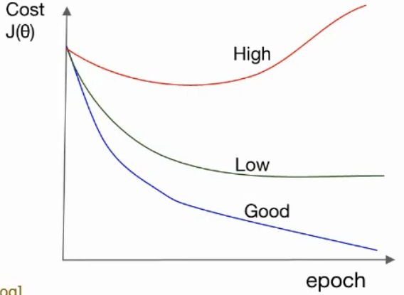
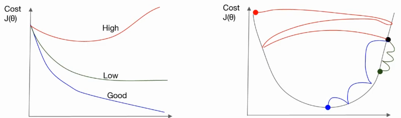
learning rate는 한 번에 얼마나 이동하는지 결정하는 값이다.
즉, learning rate가 크면 한 번에 많이 이동하고, 작으면 한 번에 작게 이동한다.

=> 학습이 잘 되면 epoch 동안 cost는 떨어진다.
=> 학습이 안 되면 cost가 점점 증가할 수 있다.
=> learning rate가 너무 크면 오버슈팅(overshooting) 현상이 발생하여 오히려 학습도가 떨어질 수 있다.
=> 반대로 너무 작으면 최적값을 찾는 시간이 너무 길어지게 된다.
=> 그래서 일반적으로 $0.01$를 많이 사용함.
=> 또는 Adam optimizer를 사용할 경우 $3\times10^{-4}$도 쓴다.

# Train Log
Iter: 0,    Loss: 6.0257, Learning Rate: 0.1000
Iter: 1000, Loss: 0.3723, Learning Rate: 0.0960
Iter: 2000, Loss: 0.2779, Learning Rate: 0.0922
Iter: 3000, Loss: 0.2293, Learning Rate: 0.0885
Iter: 4000, Loss: 0.1977, Learning Rate: 0.0849
Iter: 5000, Loss: 0.1750, Learning Rate: 0.0815


# [Tensorflow Code]
optimizer = tf.train.GradientDescentOptimizer(learning_rate=0.01)

---

1-3. Annealing the learning rate(Decay)

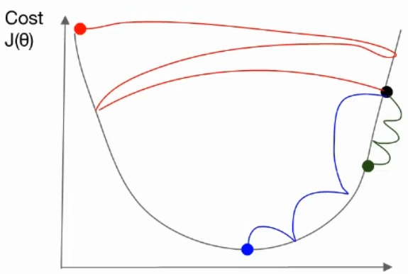
• learning rate 값을 정했다 하더라도 학습 과정에서 learning rate를 적절히 조절하는 것이 중요하다.
  = Learning rate Decay

• 학습을 하다 보면 더 이상 learning rate를 줄이지 않아도 되는 구간이 있다.
  => 이때 learning rate를 조절함으로써 cost를 더 줄일 수 있다(= decay).

종류

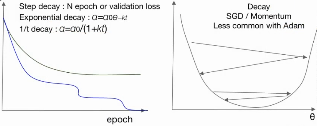
1. Step decay : $N$ epoch 또는 validation loss 기준으로 일정 스텝별 조절

2. Exponential decay : $\alpha=\alpha_0e^{-kt}$

3. 1/t decay : $\alpha=\dfrac{\alpha_0}{1+kt}$

# [Tensorflow Code]
learning_rate = tf.train.exponential_decay(
    starter_learning_rate,
    global_step,
    1000,
    0.96,
    staircase=True
)
# tf.train.exponential_decay / tf.train.inverse_time_decay
# tf.train.natural_exp_decay / tf.train.piecewise_constant
# tf.train.polynomial_decay

def exponential_decay(epoch):
    starter_rate = 0.01
    k = 0.96
    exp_rate = starter_rate * np.exp(-k * epoch)
    return exp_rate

---

2. Data preprocessing(데이터 전처리)

2-1. Feature Scaling

Feature들의 스케일을 맞춰 주는 것이 중요하다.
값의 범위가 너무 다르면 학습이 불안정해질 수 있다.

---

2-2. Standardization(표준화) / Normalization(정규화)

표준화와 정규화의 수식은 다음과 같다.

• 표준화: Standardization(Mean Distance)
  $x_{\text{new}}=\dfrac{x-\mu}{\sigma}$

• 정규화: Normalization(0–1)
  $x_{\text{new}}=\dfrac{x-x_{\min}}{x_{\max}-x_{\min}}$

# [Python Code (numpy)]
# Standardization
standardization = (data - np.mean(data, axis=0)) / np.sqrt(
    np.sum((data - np.mean(data, axis=0))**2, axis=0) / data.shape[0]
)

# Normalization (0~1)
normalization = (data - np.min(data, axis=0)) / (
    np.max(data, axis=0) - np.min(data, axis=0)
)

---

2-3. Noisy Data(쓸모없는 데이터)

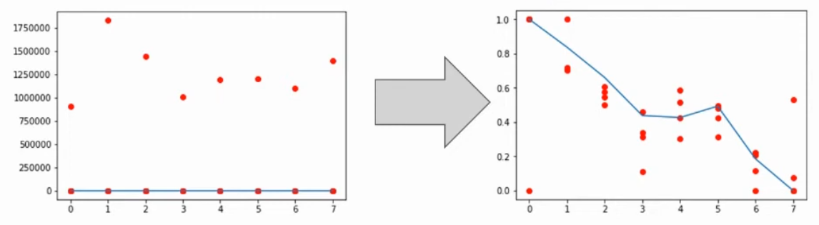
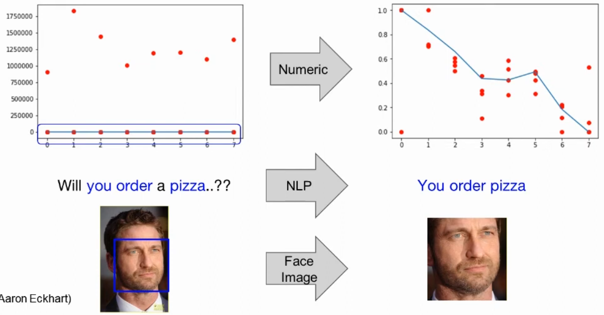
: 데이터를 잘 처리하기 위해서는 쓸모없는 데이터(노이즈 데이터)를 없애는 것이 가장 중요하다.

• 숫자 데이터 - 너무 크거나 작은 값을 제거
• NLP(자연어 처리) - 의미 있는 단어만 남기고 제거
• Face Image - 이미지 처리에 필요한 얼굴만 남김

---

3. Overfitting

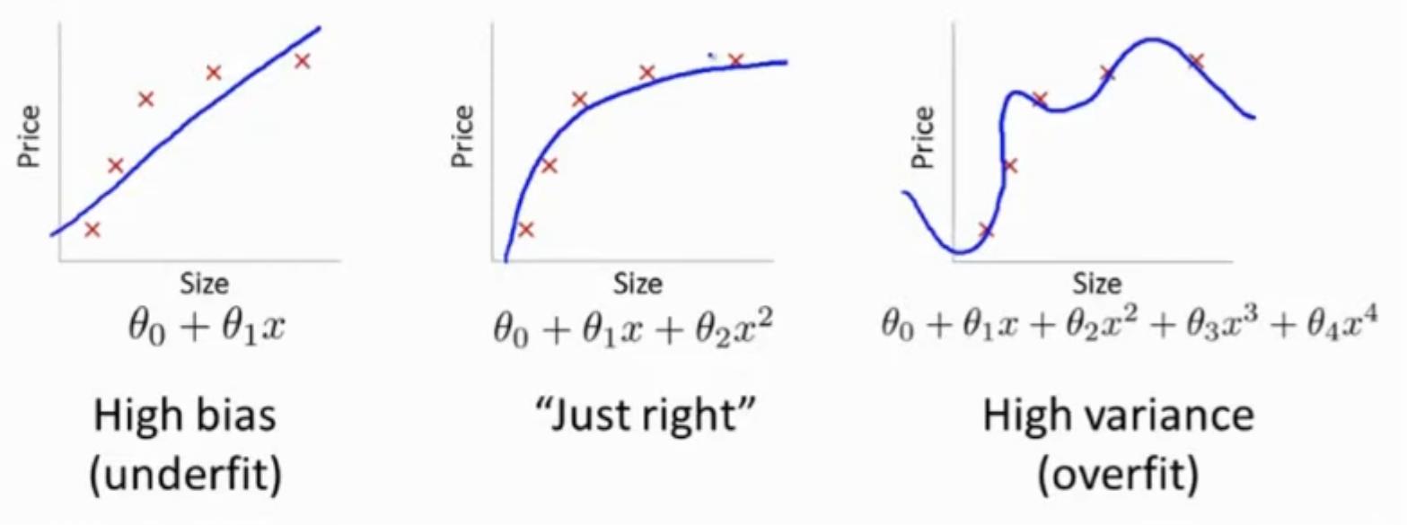
Overfitting(과적합)
: 모델이 훈련 데이터에 너무 치중되어 있는 현상(새로운 데이터 성능 저하)

• High bias(underfit)
  테스트 데이터(실제 패턴)를 반영하지 못함
• Just right
  가장 적절한 복잡도
• High variance(overfit)
  훈련 데이터에 너무 치중되어, 새로운 데이터에 약함

---

3-1. set a feature

1. 더 많은 트레이닝 데이터 투입
   데이터를 많이 넣음으로써 데이터의 다양한 변화를 반영하고, 과적합을 줄인다.
2. feature를 줄인다
   차원을 줄여서 각 데이터의 의미를 좀 더 분명히 한다(PCA).
3. feature를 더한다
   모델이 너무 심플하면 feature를 추가하여 더 특징적인 모델을 만든다.

# [sklearn Code]
from sklearn.decomposition import PCA

pca = PCA(n_components=3)
pca.fit(X)
X = pca.transform(X)

---

3-2. Regularization(정규화/규제)

: 학습 과정에서 특정 값을 추가하여 정규화(규제) 할 수 있다.
=> $\lambda$ 값을 term으로 줌으로써 해결

Linear regression with regularization

Model: $h_\theta(x)=\theta_0+\theta_1x+\theta_2x^2+\theta_3x^3+\theta_4x^4$

Cost function: $J(\theta)=\dfrac{1}{2m}\sum_{i=1}^{m}\bigl(h_\theta(x^{(i)})-y^{(i)}\bigr)^2+\dfrac{\lambda}{2m}\sum_{j=1}^{m}\theta_j^2$

=> Linear regression의 cost function에다가 $\lambda$를 줌으로써 정규화 효과를 줄 수 있다.
=> 즉, 손실 함수에 "패널티"를 추가하여 파라미터가 너무 커지거나 복잡해지지 못하게 한다.

# [Tensorflow Code]
L2_loss = tf.nn.l2_loss(w)  # output = sum(t ** 2) / 2

---

3-3. solution

Overfitting을 줄이는 대표적인 방법

• Feature Normalization
• Regularization
• more data
  • color jittering
  • horizontal flips
  • random crops/scales
• dropout
• Batch Normalization

---

4. Codes(Eager Execution) - L2 Norm

4-1. sample data

import tensorflow as tf
import numpy as np

# 예제 데이터 중간중간에 너무 큰 값들이 있다.
# => 이를 normalization을 통해 전처리 해 준다.
xy = np.array([
    [828.659973, 833.450012, 908100, 828.349976, 831.659973],
    [823.02002,  828.070007, 1828100, 821.655029, 828.070007],
    [819.929993, 824.400024, 1438100, 818.97998,  824.159973],
    [816,        820.958984, 1008100, 815.48999,  819.23999],
    [819.359985, 823,        1188100, 818.469971, 818.97998],
    [819,        823,        1198100, 816,        820.450012],
    [811.700012, 815.25,     1098100, 809.780029, 813.669983],
    [809.51001,  816.659973, 1398100, 804.539978, 809.559998]
], dtype=np.float32)

# x(입력 특징들)과 y(타깃 값)를 분리
x_train = xy[:, 0:-1]
y_train = xy[:, [-1]]

# Normalization (0~1)
# x_new = (x - x_min) / (x_max - x_min)
def normalization(data):
    # 각 열(column)별로 min-max 정규화 (0~1 구간)
    numerator = data - np.min(data, 0)
    denominator = np.max(data, 0) - np.min(data, 0)
    return numerator / denominator

xy = normalization(xy)

---

4-2. L2 Norm

Linear regression

$h_\theta(x)=\theta_0+\theta_1x+\theta_2x^2+\theta_3x^3+\theta_4x^4$

$J(\theta)=\dfrac{1}{2m}\sum_{i=1}^{m}\bigl(h_\theta(x^{(i)})-y^{(i)}\bigr)^2+\dfrac{\lambda}{2m}\sum_{j=1}^{m}\theta_j^2$

dataset = tf.data.Dataset.from_tensor_slices((x_train, y_train)).batch(len(x_train))

W = tf.Variable(tf.random_normal([4, 1]), dtype=tf.float32)
b = tf.Variable(tf.random_normal([1]), dtype=tf.float32)

# 예측값 계산
def linearReg_fn(features):
    hypothesis = tf.matmul(features, W) + b
    return hypothesis

# 실제 loss에서 정규화된 값을 구하게 된다.
def l2_loss(loss, beta=0.01):
    W_reg = tf.nn.l2_loss(W)  # output = sum(t ** 2) / 2
    loss = tf.reduce_mean(loss + W_reg * beta)
    return loss

# 실제 가설과 y값의 차이의 최소값을 구함.
# flag를 통해 적용 여부를 결정함.
# 이상치 값을 정규화 시키는 과정
def loss_fn(hypothesis, labels, flag=False):
    cost = tf.reduce_mean(tf.square(hypothesis - labels))
    if flag:
        cost = l2_loss(cost)
    return cost

---

4-3. Learning Decay

is_decay = True
starter_learning_rate = 0.1

if is_decay:
    global_step = tf.Variable(0, trainable=False)
    learning_rate = tf.train.exponential_decay(
        starter_learning_rate,  # 초기 학습률
        global_step,            # 몇 번 업데이트했는지
        50,                     # decay_steps
        0.96,                   # decay_rate
        staircase=True          # 계단식 감소 여부
    )
    optimizer = tf.train.GradientDescentOptimizer(learning_rate)
else:
    optimizer = tf.train.GradientDescentOptimizer(
        learning_rate=starter_learning_rate
    )

def grad(features, labels, l2_flag):
    with tf.GradientTape() as tape:
        loss_value = loss_fn(linearReg_fn(features), labels, l2_flag)
    return tape.gradient(loss_value, [W, b]), loss_value

for step in range(EPOCHS):
    for features, labels in tfe.Iterator(dataset):
        features = tf.cast(features, tf.float32)
        labels = tf.cast(labels, tf.float32)

        grads, loss_value = grad(features, labels, False)
        optimizer.apply_gradients(
            grads_and_vars=zip(grads, [W, b]),
            global_step=global_step
        )

    if step % 10 == 0:
        print(
            "Iter: {}, Loss: {:.4f}, Learning Rate: {:.8f}".format(
                step,
                loss_value,
                optimizer._learning_rate()
            )
        )

---

4-4. Full Code

import os
os.environ["TF_CPP_MIN_LOG_LEVEL"] = "2"  # 0: INFO, 1: WARNING, 2: ERROR, 3: FATAL
import tensorflow as tf
import numpy as np
tf.get_logger().setLevel('ERROR')

# 4-1. sample data + normalization -------------------------------------------
# 예제 데이터 중간중간에 너무 큰 값들이 있다.
# => 이를 normalization을 통해 전처리 해 준다.
xy = np.array([
    [828.659973, 833.450012, 908100, 828.349976, 831.659973],
    [823.02002,  828.070007, 1828100, 821.655029, 828.070007],
    [819.929993, 824.400024, 1438100, 818.97998,  824.159973],
    [816.,       820.958984, 1008100, 815.48999,  819.23999],
    [819.359985, 823.,       1188100, 818.469971, 818.97998],
    [819.,       823.,       1198100, 816.,       820.450012],
    [811.700012, 815.25,     1098100, 809.780029, 813.669983],
    [809.51001,  816.659973, 1398100, 804.539978, 809.559998],
], dtype=np.float32)

# x(입력 특징들)과 y(타깃 값)를 분리
x_train_raw = xy[:, 0:-1]
y_train_raw = xy[:, [-1]]


# Normalization (0~1)
# x_new = (x - x_min) / (x_max - x_min)
def normalization(data):
    # 각 열(column)별로 min-max 정규화 (0~1 구간)
    numerator = data - np.min(data, 0)
    denominator = np.max(data, 0) - np.min(data, 0)
    return numerator / denominator


# xy 전체를 normalization 한 뒤 다시 x/y를 나눠도 됨
xy_norm = normalization(xy)
x_train = xy_norm[:, 0:-1]
y_train = xy_norm[:, [-1]]

# tf.data.Dataset 구성
dataset = tf.data.Dataset.from_tensor_slices((x_train, y_train)).batch(len(x_train))


# 4-2. L2 Norm (모델, L2 loss 정의) ------------------------------------------
# 파라미터 초기화
W = tf.Variable(tf.random.normal([4, 1]), dtype=tf.float32, name="weight")
b = tf.Variable(tf.random.normal([1]), dtype=tf.float32, name="bias")


# 예측값 계산
def linearReg_fn(features):
    hypothesis = tf.matmul(features, W) + b
    return hypothesis


# 실제 loss에서 정규화된 값을 구하게 된다.
def l2_loss(loss, beta=0.01):
    # output = sum(t ** 2) / 2
    W_reg = tf.nn.l2_loss(W)
    loss = tf.reduce_mean(loss + W_reg * beta)
    return loss


# 실제 가설과 y값의 차이의 최소값을 구함.
# flag를 통해 L2 적용 여부를 결정함.
def loss_fn(hypothesis, labels, flag=False):
    cost = tf.reduce_mean(tf.square(hypothesis - labels))
    if flag:
        cost = l2_loss(cost)
    return cost


# 4-3. Learning Decay (학습 루프) -------------------------------------------
is_decay = True
starter_learning_rate = 0.1
EPOCHS = 101


if is_decay:
    lr_schedule = tf.keras.optimizers.schedules.ExponentialDecay(
        initial_learning_rate=starter_learning_rate,
        decay_steps=50,   # decay_steps=50 과 동일 의미
        decay_rate=0.96,
        staircase=True,
    )
    optimizer = tf.keras.optimizers.SGD(learning_rate=lr_schedule)
else:
    optimizer = tf.keras.optimizers.SGD(learning_rate=starter_learning_rate)


def grad(features, labels, l2_flag):
    with tf.GradientTape() as tape:
        hypothesis = linearReg_fn(features)
        loss_value = loss_fn(hypothesis, labels, l2_flag)
    grads = tape.gradient(loss_value, [W, b])
    return grads, loss_value


def train():
    for step in range(EPOCHS):
        for features, labels in dataset:
            features = tf.cast(features, tf.float32)
            labels = tf.cast(labels, tf.float32)

            grads, loss_value = grad(features, labels, l2_flag=True)
            optimizer.apply_gradients(zip(grads, [W, b]))

        if step % 10 == 0:
            # 현재 learning rate 확인 (schedule 사용 시)
            if callable(optimizer.learning_rate):
                current_lr = optimizer.learning_rate(optimizer.iterations).numpy()
            else:
                current_lr = optimizer.learning_rate.numpy()

            print(
                "Iter: {}, Loss: {:.6f}, Learning Rate: {:.8f}".format(
                    step,
                    float(loss_value.numpy()),
                    float(current_lr),
                )
            )


if __name__ == "__main__":
    print("TensorFlow version:", tf.__version__)
    train()
    print("Trained W:", W.numpy())
    print("Trained b:", b.numpy())

---

5. MNIST Classification

Fashion MNIST : 의류 데이터 분류

Sample Data

# Tensorflow Code
fashion_mnist = keras.datasets.fashion_mnist
(train_images, train_labels), (test_images, test_labels) = fashion_mnist.load_data()

class_names = ['T-shirt/top', 'Trouser', 'Pullover', 'Dress', 'Coat',
               'Sandal', 'Shirt', 'Sneaker', 'Bag', 'Ankle boot']

train_images = train_images / 255.0  # (60000, 28, 28)
test_images = test_images / 255.0    # (10000, 28, 28)

model = keras.Sequential([
    keras.layers.Flatten(input_shape=(28, 28)),
    keras.layers.Dense(128, activation=tf.nn.relu),
    keras.layers.Dense(10, activation=tf.nn.softmax)
])

model.compile(optimizer='adam',
              loss='sparse_categorical_crossentropy',
              metrics=['accuracy'])

model.fit(train_images, train_labels, epochs=5)
test_loss, test_acc = model.evaluate(test_images, test_labels)
predictions = model.predict(test_images)
np.argmax(predictions[0])  # 9 Label

---

IMDB-Text : 자연어 처리 데이터

Sample Data

# Tensorflow Code
imdb = keras.datasets.imdb
(train_data, train_labels), (test_data, test_labels) = imdb.load_data(num_words=10000)
word_index = imdb.get_word_index()
# The first indices are reserved
word_index = {k: (v + 3) for k, v in word_index.items()}
word_index["<PAD>"] = 0
word_index["<START>"] = 1
word_index["<UNK>"] = 2    # unknown
word_index["<UNUSED>"] = 3
reverse_word_index = dict([(value, key) for (key, value) in word_index.items()])

train_data = keras.preprocessing.sequence.pad_sequences(
    train_data,
    value=word_index["<PAD>"],
    padding='post',
    maxlen=256
)

model = keras.Sequential()
model.add(keras.layers.Embedding(vocab_size, 16))
model.add(keras.layers.GlobalAveragePooling1D())
model.add(keras.layers.Dense(16, activation=tf.nn.relu))
model.add(keras.layers.Dense(1, activation=tf.nn.sigmoid))
model.compile(optimizer='adam',
              loss='sparse_categorical_crossentropy',
              metrics=['accuracy'])

model.fit(partial_x_train, partial_y_train, epochs=40,
          validation_data=(x_val, y_val))

---

CIFAR-100

Sample Data

# TensorFlow Code
from keras.datasets import cifar100
(x_train, y_train), (x_test, y_test) = cifar100.load_data(label_mode='fine')

---

Summary

• Learning rate는 Gradient 방향으로 이동하는 스텝 크기를 결정한다.
• 너무 큰 learning rate는 overshooting, 너무 작은 learning rate는 느린 수렴을 만든다.
• Decay 기법으로 epoch가 진행될수록 learning rate를 줄여 더 좋은 최소값을 찾을 수 있다.
• Standardization과 Normalization으로 feature 스케일을 맞추면 학습이 안정적이다.
• Overfitting은 훈련 데이터에만 너무 맞춘 상태이며, feature 설계, Regularization, 데이터 증가 등으로 완화한다.
• L2 Regularization은 비용 함수에 $\lambda$ term을 추가해 파라미터 크기를 제약하는 대표적인 규제 방법이다.

1. Data set

1-1. Training / Validation / Testing

• 모델을 만들 때는 학습용 데이터(Training set) 와 평가용 데이터(Validation/Test set) 를 나누어 관리한다.
• 학습은 주로 Training set으로 진행하고, Validation set으로 하이퍼 파라미터를 조정하면서 우리가 원하는 성능의 모델을 만든다.
• 최종적으로는 테스트 데이터(Test set) 를 사용해 모델의 일반화 성능을 평가한다.

1-2. Evaluating a hypothesis

• 학습이 끝난 뒤, 더 이상 파라미터를 수정하지 않는 상태에서 테스트 데이터로 성능을 측정한다.
• 이때 얻은 정확도/오차가 해당 모델(가설, hypothesis)의 최종 평가 결과가 된다.

1-3. Anomaly Detection

• 이상 감지(Anomaly Detection)는 정상(normal) 데이터 위주로 학습한 뒤, 새로운 데이터가 정상 분포에서 얼마나 벗어났는지를 보고 이상 여부를 판별하는 방법이다.
• 정상 데이터만 충분히 수집할 수 있고, 이상 데이터는 드물거나 정의하기 어려운 경우에 많이 사용한다.

2. Learning

2-1. Online Learning vs Batch Learning

• Batch Learning
  • 한 번에 모아 둔 고정된 데이터셋으로 모델을 학습하는 방식.
  • 학습이 끝나면, 새로운 데이터가 많이 쌓였을 때 다시 처음부터 재학습하는 경우가 많다.
• Online Learning
  • 데이터가 실시간으로 들어오는 환경에서, 들어오는 데이터 조각마다 모델을 조금씩 업데이트하는 방식.
  • 추천 시스템, 로그 분석처럼 데이터가 계속 쌓이는 서비스에서 자주 사용된다.

2-2. Fine tuning / Feature Extraction

• Fine tuning
  • 이미 학습된 모델의 가중치를 초기값으로 사용하고, 새로운 데이터로 전체 또는 일부 레이어를 계속 학습하여 우리 데이터에 맞게 미세 조정하는 방법.
• Feature Extraction
  • 사전 학습된 모델의 앞부분을 특징 추출기(feature extractor) 로만 사용하고, 그 위에 새로운 분류기 레이어만 쌓아서 학습하는 방법.
  • 앞쪽 레이어는 고정(freeze)하고, 마지막 몇 개 레이어만 학습하는 경우가 많다.

2-3. Efficient Models

• 모델을 실제 서비스에 적용하려면 속도, 메모리, 배포 환경을 고려해 경량화가 필요하다.
• 예시
  • 파라미터 수를 줄인 작은 모델 설계
  • 모델 압축, pruning, quantization 등으로 연산량과 모델 크기 감소
  • 모바일·임베디드 환경에서도 동작 가능하게 만드는 것

3. Sample Data

• 이 강의에서는 다음과 같은 대표적인 데이터셋을 사용해 분류와 텍스트 처리 예제를 다룬다.
  • Fashion MNIST: 의류 이미지 분류(MNIST 변형 버전)
  • IMDB: 영화 리뷰 텍스트를 사용한 감성 분류(긍정/부정)
  • CIFAR-100: 100개 카테고리의 컬러 이미지 분류

---

모두를 위한 딥러닝 강좌 2
https://www.youtube.com/watch?v=7eldOrjQVi0&list=PLQ28Nx3M4Jrguyuwg4xe9d9t2XE639e5C

---

모두를 위한 딥러닝 강좌 2
https://www.youtube.com/watch?v=7eldOrjQVi0&list=PLQ28Nx3M4Jrguyuwg4xe9d9t2XE639e5C