Softmax Classifier 기본

Sample Dataset

x_data = [
	[1, 2, 1, 1],
	[2, 1, 3, 2],
	[3, 1, 3, 4],
	[4, 1, 5, 5],
	[1, 7, 5, 5],
	[1, 2, 5, 6],
	[1, 6, 6, 6],
	[1, 7, 7, 7],
]

# One-Hot encoding: 특정 부분에 대해서만 표기하고 나머지는 0으로 표기하는 방법.
y_data = [
	[0, 0, 1],
	[0, 0, 1],
	[0, 0, 1],
	[0, 1, 0],
	[0, 1, 0],
	[0, 1, 0],
	[1, 0, 0],
	[1, 0, 0],
]

# convert into numpy and float format
x_data = np.asarray(x_data, dtype=np.float32)
y_data = np.asarray(y_data, dtype=np.float32)

nb_classes = 3	# num classes

Softmax function

: 여러개의 클래스를 예측할 때 유용하다.

• $XW=Y=\begin{bmatrix}2.0\\1.0\\0.1\end{bmatrix}\ \rightarrow{\ S(y_i)=\frac{e^{y_i}}{\sum_{j} e^{y_j}}\ \rightarrow}\ \begin{bmatrix}0.7\\0.2\\0.1\end{bmatrix}$
• 이때 Softmax는 확률값으로 변환하는 과정이기 때문에 전체 확률의 총합은 항상 1이 된다.
• 코드에서는 hypothesis = tf.nn.softmax(tf.matmul(x_data, W) + b)으로 softmax를 사용하게 된다.
  • Logistic classifier의 $Y = XW$는 tf.matmul(x_data, W) + b로 구현한다.

# logistic classifier 함수인 tf.matmul(X, W) + b에 softmax 사용
# hypothesis = tf.nn.softmax(tf.matmul(X, W) + b)
		
# wieght and bias setting
# Y = XW
w = tfe.Variable(tf.random_normal([4, nb_classes]), name='weight')
b = tfe.Variable(tf.random_normal([nb_classes]), name='bias')
variables = [w, b]

hypothesis = tf.nn.softmax(tf.matmul(x_data, W) + b)

• 테스트 및 출력

# Softmax onehot test
sample_db = [[8,2,1,4]]
ample_db = np.asarray(sample_db, dtype=np.float32)

# Test output
# tf.Tensor([[0.9302204  0.06200533 0.00777428]], shape=(1, 3), dtype=float32)

Cost function

# Cross entropy cost/loss
cost = tf.reduce_mean(-tf.reduce_sum(Y * tf.log(hypothesis), axis=1))

optimizer = tf.train.GradientDescentOptimizer(learning_rate=0.1).minimize(cost)
		
def cost_fn(X, Y):
	logits = hypothesis(X)
	cost = -tf.reduce_sum(Y * tf.log(logits), axis=1)
	cost_mean = tf.reduce_mean(cost)
	return cost_mean

print(cost_fn(x_data, y_data))

• 테스트 및 출력

# Cost 출력
tf.Tensor(
[3.4761162e+00 8.2235537e+00 6.6874886e+00 6.9770794e+00 6.4782157e+00
 3.7971997e+00 8.9059100e-03 6.9166054e-03], shape=(8,), dtype=float32)

# Cost mean 출력
tf.Tensor(4.4569345, shape=(), dtype=float32)

Gradiant function

def grad_fn(X, Y):
	with tf.GradientTape() as tape:
		cost = cost_fn(X, Y)
	grads = tape.gradient(cost, variables)
	return grads

print(grad_fn(x_data, y_data))

• 테스트 및 출력

[(<tf.Tensor: id=533, shape=(4, 3), dtype=float32, numpy=
array([[ 0.06991257, -0.00614021, -0.06377237],
	   [ 0.02443989, -0.00085829, -0.02358155],
	   [ 0.06863485, -0.01986565, -0.04876918],
	   [ 0.08595259, -0.01490254, -0.07105   ]], dtype=float32)>,
 <tf.Tensor: id=531, shape=(3,), dtype=float32, numpy=array([ 0.02441996,  0.00028941, -0.02470937], dtype=float32)>]

Train & Result

def fit(X, Y, epochs=2000, verbose=100):
	optimizer = tf.train.GradientDescentOptimizer(learning_rate=0.1)
	for i in range(epochs):
		grads = grad_fn(X, Y)
		optimizer.apply_gradients(zip(grads, variables))
		if (i==0) | ((i+1)%verbose==0):
			print('Loss at epoch %d: %f' %(i+1, cost_fn(X,Y).numpy()))

• 테스트 및 출력

# log 출력
Loss at epoch 100: 0.153950
Loss at epoch 200: 0.148822
...
Loss at epoch 1900: 0.094386
Loss at epoch 2000: 0.092371
# => loss가 점점 0에 가까워진다. = 더 정확해진다.

Predict

a = hypothesis(x_data)

print(a)
print(tf.argmax(a, 1))
print(tf.argmax(y_data, 1))  # matches with y_data

• 테스트 및 출력

# 최종 결과 출력
tf.Tensor(
[[1.5791884e-09 1.2361944e-06 9.9999881e-01]
 [3.4672192e-03 2.1560978e-02 9.7497183e-01]
 [2.7782797e-11 2.3855740e-02 9.7614425e-01]
 [2.1569745e-08 8.3984965e-01 1.6015036e-01]
 [5.1191613e-02 9.3995154e-01 8.8568293e-03]
 [2.9994551e-02 9.7000545e-01 6.1867158e-18]
 [9.0973479e-01 9.0265274e-02 8.0962785e-11]
 [9.7926140e-01 2.0738611e-02 7.9181873e-14]], shape=(8, 3), dtype=float32)
# 각 dataset에 대한 예측값을 나타낸다.
# 0번 : [0.00000015791884%, 0.00012361944%, 99.999881%] 
# 1번 : [0.34672192%, 2.1560978%, 97.497183%]
# 2번 : [0.0000000027782797%, 2.385574%, 97.614425%]
# ...
# 7번 : [2.9994551%, 97.000545%, 6.1867158000e-16%]
# 8번 : [90.973479%, 9.0265274%, 0.0000000080962785%]
# => 즉, 각 클래스별 확률이 되고, 가장 확률이 높은 것을 선택하게 된다.


tf.Tensor([2 2 2 1 1 1 0 0], shape=(8,), dtype=int64)
tf.Tensor([2 2 2 1 1 1 0 0], shape=(8,), dtype=int64)

전체 코드

import tensorflow as tf
import numpy as np
tf.get_logger().setLevel('ERROR')

# 1. 데이터 정의 (사용자 코드 유지)
x_data = [
    [1, 2, 1, 1],
    [2, 1, 3, 2],
    [3, 1, 3, 4],
    [4, 1, 5, 5],
    [1, 7, 5, 5],
    [1, 2, 5, 6],
    [1, 6, 6, 6],
    [1, 7, 7, 7],
]

# One-Hot encoding: 특정 부분에 대해서만 표기하고 나머지는 0으로 표기하는 방법.
y_data = [
    [0, 0, 1],
    [0, 0, 1],
    [0, 0, 1],
    [0, 1, 0],
    [0, 1, 0],
    [0, 1, 0],
    [1, 0, 0],
    [1, 0, 0],
]

# convert into numpy and float format
x_data = np.asarray(x_data, dtype=np.float32)
y_data = np.asarray(y_data, dtype=np.float32)

nb_classes = 3  # num classes

# 2. 가중치, 편향 정의
w = tf.Variable(tf.random.normal([4, nb_classes]), name='weight')
b = tf.Variable(tf.random.normal([nb_classes]), name='bias')     
variables = [w, b]

# 3. 가설 함수 정의
def hypothesis(X):
    # X: (batch_size, 4)
    logits = tf.matmul(X, w) + b
    return tf.nn.softmax(logits)

# 4. 비용 함수 정의
def cost_fn(X, Y):
    logits = hypothesis(X)  # (batch_size, nb_classes)
    # one-hot cross entropy
    # Y: one-hot 레이블, logits: softmax 확률
    cost = -tf.reduce_sum(Y * tf.math.log(logits + 1e-7), axis=1)
    cost_mean = tf.reduce_mean(cost)
    return cost_mean

# 5. 기울기 계산 함수
def grad_fn(X, Y):
    with tf.GradientTape() as tape:
        cost = cost_fn(X, Y)
    grads = tape.gradient(cost, variables)
    return grads

# 6. 학습 함수
def fit(X, Y, epochs=2000, verbose=100):
    optimizer = tf.keras.optimizers.SGD(learning_rate=0.1)

    for i in range(epochs):
        grads = grad_fn(X, Y)
        # grads: [dw, db], variables: [w, b]
        optimizer.apply_gradients(zip(grads, variables))

        if (i == 0) or ((i + 1) % verbose == 0):
            # .numpy()로 현재 cost 값을 출력
            print('Loss at epoch %d: %f' % (i + 1, cost_fn(X, Y).numpy()))

# 7. 학습 실행
fit(x_data, y_data, epochs=2000, verbose=100)

# 8. 학습된 모델로 예측 확인
a = hypothesis(x_data)

print(a)                      # 각 샘플에 대한 [class0, class1, class2] 확률
print(tf.argmax(a, 1))        # 예측된 class index
print(tf.argmax(y_data, 1))   # 실제 정답 class index (one-hot → index)

# 9. 새로운 입력(sample_db)에 대한 softmax 예측
sample_db = [[8, 2, 1, 4]]
sample_db = np.asarray(sample_db, dtype=np.float32)

print(hypothesis(sample_db))  # 예: tf.Tensor([[0.93, 0.06, 0.007]], ...)

• 출력 결과

# 각 에폭시별 loss값
Loss at epoch 1: 2.043797
Loss at epoch 100: 0.683173
Loss at epoch 200: 0.605817
Loss at epoch 300: 0.554164
Loss at epoch 400: 0.507361
Loss at epoch 500: 0.462262
Loss at epoch 600: 0.417786
Loss at epoch 700: 0.373436
Loss at epoch 800: 0.329056
Loss at epoch 900: 0.285247
Loss at epoch 1000: 0.247555
Loss at epoch 1100: 0.231185
Loss at epoch 1200: 0.220295
Loss at epoch 1300: 0.210344
Loss at epoch 1400: 0.201215
Loss at epoch 1500: 0.192811
Loss at epoch 1600: 0.185051
Loss at epoch 1700: 0.177865
Loss at epoch 1800: 0.171194
Loss at epoch 1900: 0.164984
Loss at epoch 2000: 0.159192
# => loss가 점점 줄어드는것을 볼 수 있다.

# 각 학습 데이터에 대한 예측 확률.
tf.Tensor(
[[1.8063469e-06 1.4325111e-03 9.9856573e-01]
 [4.2200583e-04 7.7052422e-02 9.2252558e-01]
 [1.3354445e-07 1.6016665e-01 8.3983326e-01]
 [2.3653492e-06 8.5565048e-01 1.4434719e-01]
 [2.6483569e-01 7.2364306e-01 1.1521227e-02]
 [1.4009903e-01 8.5975951e-01 1.4149565e-04]
 [7.3494178e-01 2.6498711e-01 7.1051436e-05]
 [9.2451102e-01 7.5487778e-02 1.1960639e-06]], shape=(8, 3), dtype=float32)

# 학습 데이터에 대한 예측값과 정답. 100% 정확하다.
tf.Tensor([2 2 2 1 1 1 0 0], shape=(8,), dtype=int64)
tf.Tensor([2 2 2 1 1 1 0 0], shape=(8,), dtype=int64)

# 새로운 데이터에 대한 예측값.
tf.Tensor([[3.2441543e-27 6.5584864e-08 9.9999988e-01]], shape=(1, 3), dtype=float32)
# 2번 클래스일 확률이 99.99%로 예측하고 있는 것을 볼 수 있다.

Softmax Classifier (Animal Classification)

Softmax function

# 위와 동일
#Weight and bias setting
W = tfe.Variable(tf.random_normal([16, nb_classes]), name='weight')
b = tfe.Variable(tf.random_normal([nb_classes]), name='bias')
variables = [W, b]

# tf.nn.softmax computes softmax activations
def logit_fn(X):
    return tf.matmul(X, W) + b

def hypothesis(X):
    return tf.nn.softmax(logit_fn(X))

Softmax cross entropy (with logits)

logits = tf.matmul(X, W) + b
hypothesis = tf.nn.softmax(logits)

# 1) Cross entropy cost/loss
cost = tf.reduce_mean(-tf.reduce_sum(Y * tf.log(hypothesis), axis=1))

# 2) Cross entropy cost/loss
cost_i = tf.nn.softmax_cross_entropy_with_logits_v2(logits=logits, labels=Y_one_hot)
cost = tf.reduce_mean(cost_i)

Sample Dataset

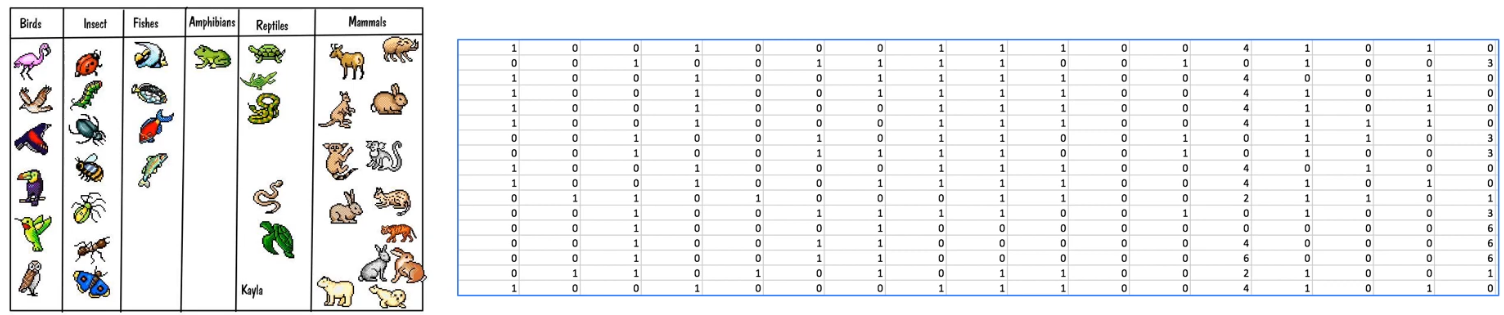
# 동물에 대한 특징을 추출하여 어떤 동물인지 예측하는 데이터이다.
# Predicting animal type based on various features
# numpy 라이브러리를 활용하여 .csv 파일을 로드한다.
xy = np.loadtxt('data-04-zoo.csv', delimiter=',', dtype=np.float32)
x_data = xy[:, 0:-1]
y_data = xy[:, [-1]]

# 우리는 ont-hot 데이터를 원하지만, 이 데이터셋은 one-hot 되어있지 않다. 
# tf.one_hot으로 변환 필요
nb_classes = 7  # 0 ~ 6

Y_one_hot = tf.one_hot(list(y_data), nb_classes)  # one hot shape=(?, 1, 7)
Y_one_hot = tf.reshape(Y_one_hot, [-1, nb_classes])  # shape=(?, 7)

# 즉, y_data가 (N, 1) 형태의 정수 라벨(스칼라)이므로, tf.one_hot(indices, depth)를 통해 각 스칼라 라벨을 길이 depth의 벡터로 치환하게 된다.
# 이 스칼라 -> 벡터 변환 과정에서 축이 하나 더 생기게 되므로, (N, 1, nb_classes)가 된다.
# 원-핫은 (N, nb_classes)의 형태로 사용하므로, tf.one_hot의 결과와는 맞지 않다. 따라서 tf.reshape()로 필요한 형태를 맞춰주게 된다.
# 코드에서 tf.reshape(Y_one_hot, [-1, nb_classes])는 nb_classes 자리를 고정하고, 앞쪽의 축을 하나의 축으로 합치게 된다.
# 결과적으로 이 코드를 통해 (?, 7)의 형태를 가지게 된다.

Cost function

def cost_fn(X, Y):
    logits = logit_fn(X)
    cost_i = tf.nn.softmax_cross_entropy_with_logits_v2(logits=logits,
                                                        labels=Y)
    cost = tf.reduce_mean(cost_i)
    return cost

Gradiant function

def grad_fn(X, Y):
    with tf.GradientTape() as tape:
        loss = cost_fn(X, Y)
        grads = tape.gradient(loss, variables)
        return grads

def prediction(X, Y):
    pred = tf.argmax(hypothesis(X), 1)
    correct_prediction = tf.equal(pred, tf.argmax(Y, 1))
    accuracy = tf.reduce_mean(tf.cast(correct_prediction, tf.float32))

    return accuracy

Train & Result

def fit(X, Y, epochs=500, verbose=50):
    optimizer = tf.train.GradientDescentOptimizer(learning_rate=0.1)

    for i in range(epochs):
        grads = grad_fn(X, Y)
        optimizer.apply_gradients(zip(grads, variables))
        if (i==0) | ((i+1)%verbose==0):
            acc  = prediction(X, Y).numpy()
            loss = tf.reduce_sum(cost_fn(X, Y)).numpy()
            print('Loss & Acc at {} epoch {}, {}'.format(i+1, loss, acc))

fit(x_data, Y_one_hot)

전체 코드

import tensorflow as tf
import numpy as np
tf.get_logger().setLevel('ERROR')

# 1) Sample Dataset 로드 (로컬 파일 사용)
xy = np.loadtxt('data-04-zoo.csv', delimiter=',', dtype=np.float32)
x_data = xy[:, 0:-1]      # (N, 16)
y_data = xy[:, [-1]]      # (N, 1)

nb_classes = 7  # 0 ~ 6

# (N, 1) 정수 라벨 → (N,) → one_hot (N, 7)
Y_one_hot = tf.one_hot(tf.squeeze(tf.cast(y_data, tf.int32), axis=1), depth=nb_classes)
Y_one_hot = tf.reshape(Y_one_hot, [-1, nb_classes])

# 2) 파라미터 정의
W = tf.Variable(tf.random.normal([16, nb_classes]), name='weight')
b = tf.Variable(tf.random.normal([nb_classes]), name='bias')
variables = [W, b]

# 3) 모델/손실/평가 함수
def logit_fn(X):
    return tf.matmul(X, W) + b

def hypothesis(X):
    return tf.nn.softmax(logit_fn(X))

def cost_fn(X, Y):
    logits = logit_fn(X)
    cost_i = tf.nn.softmax_cross_entropy_with_logits(labels=Y, logits=logits)
    cost = tf.reduce_mean(cost_i)
    return cost

def grad_fn(X, Y):
    with tf.GradientTape() as tape:
        loss = cost_fn(X, Y)
    grads = tape.gradient(loss, variables)
    return grads  # [dW, db]

def prediction(X, Y):
    pred = tf.argmax(hypothesis(X), axis=1)
    correct_prediction = tf.equal(pred, tf.argmax(Y, axis=1))
    accuracy = tf.reduce_mean(tf.cast(correct_prediction, tf.float32))
    return accuracy

# 4) 학습 루프
optimizer = tf.keras.optimizers.SGD(learning_rate=0.1)

def fit(X, Y, epochs=500, verbose=50):
    for i in range(epochs):
        grads = grad_fn(X, Y)
        optimizer.apply_gradients(zip(grads, variables))
        if (i == 0) | ((i + 1) % verbose == 0):
            acc  = prediction(X, Y).numpy()
            loss = tf.reduce_sum(cost_fn(X, Y)).numpy()
            print('Loss & Acc at {} epoch {}, {}'.format(i + 1, loss, acc))

# 5) 실행
fit(x_data, Y_one_hot)

• 출력 결과

Loss & Acc at 1 epoch 9.503366470336914, 0.019801979884505272
Loss & Acc at 50 epoch 0.7734508514404297, 0.7326732873916626
Loss & Acc at 100 epoch 0.4671158790588379, 0.8613861203193665
Loss & Acc at 150 epoch 0.3549104332923889, 0.9207921028137207
Loss & Acc at 200 epoch 0.29218873381614685, 0.9207921028137207
Loss & Acc at 250 epoch 0.25077736377716064, 0.9603960514068604
Loss & Acc at 300 epoch 0.22084419429302216, 0.9603960514068604
Loss & Acc at 350 epoch 0.1979331225156784, 0.9603960514068604
Loss & Acc at 400 epoch 0.1796892136335373, 0.9801980257034302
Loss & Acc at 450 epoch 0.16473577916622162, 0.9900990128517151
Loss & Acc at 500 epoch 0.152207612991333, 0.9900990128517151

출처: 모두를 위한 딥러닝 강좌 2
https://www.youtube.com/watch?v=7eldOrjQVi0&list=PLQ28Nx3M4Jrguyuwg4xe9d9t2XE639e5C