Lec-09 special

1. 미분의 정의

$\dfrac{d}{dx}f(x)=\lim_{\Delta x\to 0}\dfrac{f(x+\Delta x)-f(x)}{\Delta x}$

이를 다른 말로, 순간변화율이라고 한다.

이제, 다음 예제들을 생각해 보자.
(단, 편의상 $\Delta x=0.01$ 이라고 하자.)

---

2. 예제로 보는 미분

2-1) $f(x)=3$

=> 이 함수의 경우, $x$의 값에 상관없이 항상 3을 출력한다.

$\dfrac{f(x+0.01)-f(x)}{0.01}=\dfrac{3-3}{0.01}=0$

=> 즉, 상수 함수를 미분하면 0이 나온다.

---

2-2) $f(x)=x$

$\dfrac{f(x+0.01)-f(x)}{0.01}=\dfrac{(x+0.01)-x}{0.01}=\dfrac{0.01}{0.01}=1$

=> $\dfrac{dx}{dx}=1$

---

2-3) $f(x)=2x$

$\dfrac{f(x+0.01)-f(x)}{0.01}=\dfrac{2(x+0.01)-2x}{0.01}=\dfrac{2x+0.02-2x}{0.01}=\dfrac{0.02}{0.01}=2$

---

3. Partial derivative (편미분)

: 내가 관심있는 변수 외의 다른 변수는 상수로 취급한다.

1) $f(x,y)=xy,\ \dfrac{\partial f}{\partial x}=y$

2) $f(x,y)=xy,\ \dfrac{\partial f}{\partial y}=x$

3) $f(x)=2x\Rightarrow f(x)=x+x$

=> $\dfrac{df}{dx}=\dfrac{dx}{dx}+\dfrac{dx}{dx}=1+1=2$

4) $f(x)=x+3$

=> $\dfrac{df}{dx}=1+0$

5) $f(x,y)=x+y$

=> $\dfrac{\partial f}{\partial x}=1+0$

6) $f(x,y)=x+y$

=> $\dfrac{\partial f}{\partial y}=0+1$

---

4. compound function (복합함수)

ex) $z=wx+b,\ h=\text{sig}(z)$ 와 같은 경우,
우리가 원하는 건 $x$가 $h$에 미치는 영향이다.

1) $f(g(x))$

연쇄법칙(chain rule)

$\dfrac{\partial f}{\partial x}=\dfrac{\partial f}{\partial g}\cdot\dfrac{\partial g}{\partial x}$

=> 1. $f$를 $g$로 미분
=> 2. $g$를 $x$로 미분

---

Lec-09 1, 2

XOR 문제 딥러닝으로 풀기 (Neural Network for XOR)

---

1. XOR 문제와 로지스틱 회귀

하나의 로지스틱 회귀 유닛으로는 XOR을 구분할 수 없다.
=> 하나가 아닌 여러 개의 유닛을 사용하면 풀 수 있다.
=> 그러나 Neural Network(NN) 없이 하나의 선으로는 분리가 안 된다.

1-1. XOR 진리표

x1	x2	XOR
0	0	0 (-)
0	1	1 (+)
1	0	1 (+)
1	1	0 (-)

---

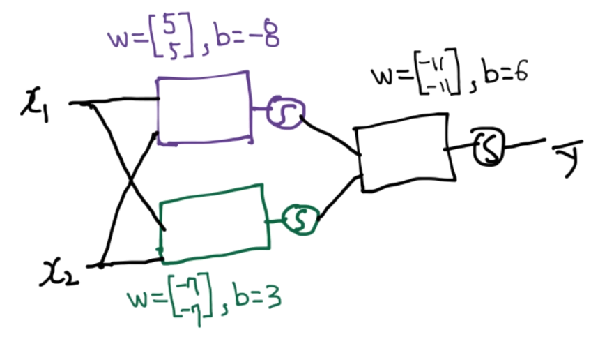
2. XOR using NN (3개의 NN 사용)

NN = 하나의 네트워크(유닛)는 하나의 로지스틱 회귀와 같다.

• 입력: 2개 $(x_1,x_2)$
• 내부 연산: $WX+b$
• 활성화 함수: sigmoid
• 출력: 1개

각 유닛의 $w,b$를 다음과 같이 가정하자.

• NN1 : $x_1,x_2\Rightarrow W=[5,5],\ b=-8\Rightarrow y_1$
• NN2 : $x_1,x_2\Rightarrow W=[-7,-7],\ b=3\Rightarrow y_2$
• NN3 : $y_1,y_2\Rightarrow W=[-11,-11],\ b=6\Rightarrow \bar{y}$

---

2-1. case 1 : $x_1=0,\ x_2=0$ (XOR=0)

• NN1

  $z_1=[0,0]\begin{bmatrix}5\\5\end{bmatrix}-8=-8$
  $y_1=S(-8)\approx 0$

• NN2

  $z_2=[0,0]\begin{bmatrix}-7\\-7\end{bmatrix}+3=3$
  $y_2=S(3)\approx 1$

• NN3

  $z_3=[0,1]\begin{bmatrix}-11\\-11\end{bmatrix}+6=-5$
  $\bar{y}=S(-5)\approx 0$

• 정리

x1	x2	y1	y2	$\bar{y}$	XOR
0	0	0	1	0	0 (-) (correct)

---

2-2. case 2 : $x_1=0,\ x_2=1$ (XOR=1)

• NN1

  $z_1=[0,1]\begin{bmatrix}5\\5\end{bmatrix}-8=5-8=-3$
  $y_1=S(-3)\approx 0$

• NN2

  $z_2=[0,1]\begin{bmatrix}-7\\-7\end{bmatrix}+3=-7+3=-4$
  $y_2=S(-4)\approx 0$

• NN3

  $z_3=[0,0]\begin{bmatrix}-11\\-11\end{bmatrix}+6=6$
  $\bar{y}=S(6)\approx 1$

• 정리

x1	x2	y1	y2	$\bar{y}$	XOR
0	1	0	0	1	1 (+) (correct)

---

2-3. case 3 : $x_1=1,\ x_2=0$ (XOR=1)

• NN1

  $z_1=[1,0]\begin{bmatrix}5\\5\end{bmatrix}-8=5-8=-3$
  $y_1=S(-3)\approx 0$

• NN2

  $z_2=[1,0]\begin{bmatrix}-7\\-7\end{bmatrix}+3=-7+3=-4$
  $y_2=S(-4)\approx 0$

• NN3

  $z_3=[0,0]\begin{bmatrix}-11\\-11\end{bmatrix}+6=6$
  $\bar{y}=S(6)\approx 1$

• 정리

x1	x2	y1	y2	$\bar{y}$	XOR
1	0	0	0	1	1 (+) (correct)

---

2-4. case 4 : $x_1=1,\ x_2=1$ (XOR=0)

• NN1

  $z_1=[1,1]\begin{bmatrix}5\\5\end{bmatrix}-8=10-8=2$
  $y_1=S(2)\approx 1$

• NN2

  $z_2=[1,1]\begin{bmatrix}-7\\-7\end{bmatrix}+3=-7-7+3=-11$
  $y_2=S(-11)\approx 0$

• NN3

  $z_3=[1,0]\begin{bmatrix}-11\\-11\end{bmatrix}+6=-11+6=-5$
  $\bar{y}=S(-5)\approx 0$

• 정리

x1	x2	y1	y2	$\bar{y}$	XOR
1	1	1	0	0	0 (-) (correct)

---

2-5. 전체 결과 정리

x1	x2	y1	y2	$\bar{y}$	XOR
0	0	0	1	0	0 (-)
0	1	0	0	1	1 (+)
1	0	0	0	1	1 (+)
1	1	1	0	0	0 (-)

=> all $\bar{y}=$ XOR = correct

---

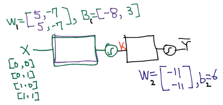
3. 2개의 유닛을 하나의 층으로 합치기

그림 느낌

• $x_1\rightarrow$ NN1 $(w=[5],b=-8)$
• $x_2\rightarrow$ NN2 $(w=[-7],b=3)$
• 두 출력이 NN3 $(w=[-11,-11],b=6)$으로 들어감

=> 2개의 유닛을 하나의 hidden layer로 합칠 수 있다.
=> Multinomial Classification(다중 클래스 분류, Lec-06 1)과 비슷한 구조.

수식으로 정리하면

• 입력 벡터: $X$

• 첫 번째 레이어:

  $K(X)=\text{Sigmoid}(XW_1+B_1)$

• 두 번째 레이어(최종 출력):

  $Y_{\text{bar}}=H(X)=\text{Sigmoid}(K(X)W_2+B_2)$

# NN 개념 정리용

K = tf.sigmoid(tf.matmul(X, W1) + b1)
hypothesis = tf.sigmoid(tf.matmul(K, W2) + b2)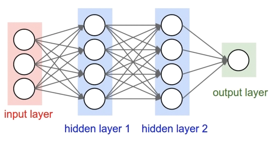

---

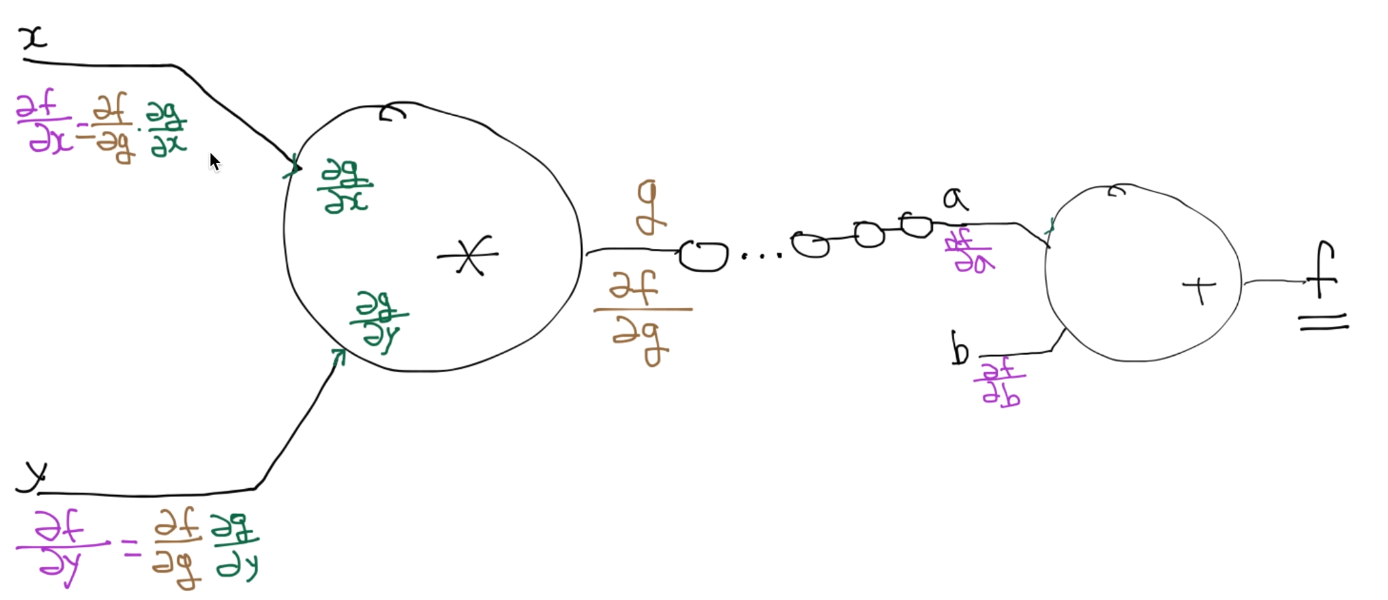
4. BackPropagation (chain rule)

$f=wx+b,\ g=wx,\ f=g+b$ 라고 하자.

• $g$에 대해

  • $\dfrac{\partial g}{\partial w}=x$
  • $\dfrac{\partial g}{\partial x}=w$

• $f$에 대해

  • $\dfrac{\partial f}{\partial g}=1$
  • $\dfrac{\partial f}{\partial b}=1$

연쇄법칙으로

• $\dfrac{\partial f}{\partial w}=\dfrac{\partial f}{\partial g}\cdot\dfrac{\partial g}{\partial w}=1\cdot x=x$
• $\dfrac{\partial f}{\partial x}=\dfrac{\partial f}{\partial g}\cdot\dfrac{\partial g}{\partial x}=1\cdot w=w$

---

4-1. forward / backward 예시

1. forward (예: $w=-2,\ x=5,\ b=3$)

• $g=wx=-10$
• $f=g+b=-7$

이때,

• $\dfrac{\partial f}{\partial g}=1$
• $\dfrac{\partial f}{\partial w}=1\cdot x=5$
  • $w$가 1 바뀌면 $f$는 5만큼 바뀐다.
• $\dfrac{\partial f}{\partial x}=1\cdot w=-2$
  • $x$가 1 바뀌면 $f$는 -2만큼 바뀐다.

2. backward

• 마지막 노드(출력 $f$)에서부터, 결과값을 알고 있으니

• 출력에서 거꾸로 미분값을 전파하면서 각 $w,x,b$를 업데이트한다.

  => BackPropagation(오차역전파)의 기본 아이디어.

---

Lec-09 1, 2 Code

XOR 문제

---

1. remind Logistic Regression

값 $X$를 넣으면

• Linear function
• logistic function (sigmoid 함수)

를 거쳐, $0\le y\le 1$ 사이의 결과로 만들 수 있다.

=> 여기에 기준값인 decision boundary를 적용하여
=> 0과 1의 값을 가지는 분류를 만들 수 있다.

XOR 문제의 경우, 이러한 2진 분류(logistic regression)만으로는 풀 수 없다.
=> 그럼 더 많은 logistic으로 풀면 어떨까?

=> 3개의 logistic regression을 사용하여 XOR을 풀 수 있다.

---

2. Neural Network

2-1. 2 layer Neural Net

• 1개의 hidden layer
• 1개의 output layer

로 구성된 network를 통해 XOR 문제를 풀 수 있다.

• hidden layer: 2개의 logistic function
• output layer: 1개의 logistic function

---

3. Vector로 합치기

hidden layer의 2개의 logistic function을 하나의 vector로 합칠 수 있다.
=> 각 logistic의 $w,b$를 하나의 벡터로 합친다.

---

4. Codes (TensorFlow 2 기준 코드)

4-1. 간단한 2-layer XOR NN (TF2, 2개의 로지스틱 유닛 + output 1개)

import tensorflow as tf

# 재현성을 위한 시드 고정
tf.random.set_seed(777)

# XOR 데이터
x_data = tf.constant([[0., 0.],
                      [0., 1.],
                      [1., 0.],
                      [1., 1.]], dtype=tf.float32)

y_data = tf.constant([[0.],
                      [1.],
                      [1.],
                      [0.]], dtype=tf.float32)

# Dataset 구성
dataset = tf.data.Dataset.from_tensor_slices((x_data, y_data)).batch(len(x_data))


def preprocess_data(features, labels):
    features = tf.cast(features, tf.float32)
    labels = tf.cast(labels, tf.float32)
    return features, labels


# 가중치 / 편향 (TF2 스타일)
W1 = tf.Variable(tf.random.normal([2, 1]), name="weight1")
b1 = tf.Variable(tf.random.normal([1]), name="bias1")

W2 = tf.Variable(tf.random.normal([2, 1]), name="weight2")
b2 = tf.Variable(tf.random.normal([1]), name="bias2")

W3 = tf.Variable(tf.random.normal([2, 1]), name="weight3")
b3 = tf.Variable(tf.random.normal([1]), name="bias3")


def neural_net(features):
    # 첫 번째 로지스틱 유닛
    layer1 = tf.sigmoid(tf.matmul(features, W1) + b1)
    # 두 번째 로지스틱 유닛
    layer2 = tf.sigmoid(tf.matmul(features, W2) + b2)
    # 두 유닛의 출력을 concat
    layer = tf.concat([layer1, layer2], axis=-1)  # shape: [batch, 2]
    # 최종 출력
    hypothesis = tf.sigmoid(tf.matmul(layer, W3) + b3)
    return hypothesis


def loss_fn(hypothesis, labels):
    # Binary cross entropy
    cost = -tf.reduce_mean(
        labels * tf.math.log(hypothesis + 1e-7)
        + (1.0 - labels) * tf.math.log(1.0 - hypothesis + 1e-7)
    )
    return cost


optimizer = tf.keras.optimizers.SGD(learning_rate=0.01)


def accuracy_fn(hypothesis, labels):
    predicted = tf.cast(hypothesis > 0.5, dtype=tf.float32)
    accuracy = tf.reduce_mean(tf.cast(tf.equal(predicted, labels), dtype=tf.float32))
    return accuracy


@tf.function
def train_step(features, labels):
    with tf.GradientTape() as tape:
        hypothesis = neural_net(features)
        loss_value = loss_fn(hypothesis, labels)
    grads = tape.gradient(loss_value, [W1, W2, W3, b1, b2, b3])
    optimizer.apply_gradients(zip(grads, [W1, W2, W3, b1, b2, b3]))
    return loss_value


EPOCHS = 50000

for step in range(EPOCHS):
    for features, labels in dataset:
        features, labels = preprocess_data(features, labels)
        loss_value = train_step(features, labels)

    if step % 5000 == 0:
        print(f"Iter: {step}, Loss: {loss_value.numpy():.4f}")

# 최종 정확도 확인
x_test, y_test = preprocess_data(x_data, y_data)
test_hypothesis = neural_net(x_test)
test_acc = accuracy_fn(test_hypothesis, y_test)
print(f"Testset Accuracy: {test_acc.numpy():.4f}")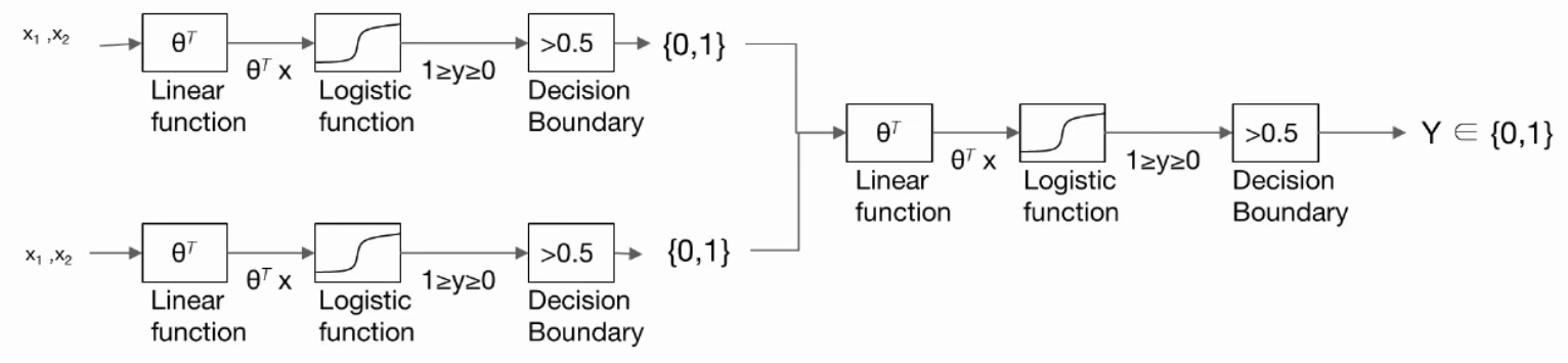

---

4-2. Vector 형태의 2-layer XOR NN (TF2)

import tensorflow as tf

tf.random.set_seed(777)

# XOR 데이터
x_data = tf.constant([[0., 0.],
                      [0., 1.],
                      [1., 0.],
                      [1., 1.]], dtype=tf.float32)

y_data = tf.constant([[0.],
                      [1.],
                      [1.],
                      [0.]], dtype=tf.float32)

dataset = tf.data.Dataset.from_tensor_slices((x_data, y_data)).batch(len(x_data))


def preprocess_data(features, labels):
    return tf.cast(features, tf.float32), tf.cast(labels, tf.float32)


# W1: [2, 2], b1: [2]  → hidden layer (뉴런 2개)
W1 = tf.Variable(tf.random.normal([2, 2]), name="weight1")
b1 = tf.Variable(tf.random.normal([2]), name="bias1")

# W2: [2, 1], b2: [1]  → output layer
W2 = tf.Variable(tf.random.normal([2, 1]), name="weight2")
b2 = tf.Variable(tf.random.normal([1]), name="bias2")


def neural_net(features):
    layer = tf.sigmoid(tf.matmul(features, W1) + b1)   # hidden layer
    hypothesis = tf.sigmoid(tf.matmul(layer, W2) + b2) # output layer
    return hypothesis


def loss_fn(hypothesis, labels):
    cost = -tf.reduce_mean(
        labels * tf.math.log(hypothesis + 1e-7)
        + (1.0 - labels) * tf.math.log(1.0 - hypothesis + 1e-7)
    )
    return cost


optimizer = tf.keras.optimizers.SGD(learning_rate=0.1)


@tf.function
def train_step(features, labels):
    with tf.GradientTape() as tape:
        hypothesis = neural_net(features)
        loss_value = loss_fn(hypothesis, labels)
    grads = tape.gradient(loss_value, [W1, W2, b1, b2])
    optimizer.apply_gradients(zip(grads, [W1, W2, b1, b2]))
    return loss_value


def accuracy_fn(hypothesis, labels):
    predicted = tf.cast(hypothesis > 0.5, dtype=tf.float32)
    accuracy = tf.reduce_mean(tf.cast(tf.equal(predicted, labels), dtype=tf.float32))
    return accuracy


EPOCHS = 10000

for step in range(EPOCHS):
    for features, labels in dataset:
        features, labels = preprocess_data(features, labels)
        loss_value = train_step(features, labels)
    if step % 1000 == 0:
        print(f"Iter: {step}, Loss: {loss_value.numpy():.4f}")

x_test, y_test = preprocess_data(x_data, y_data)
test_hypothesis = neural_net(x_test)
test_acc = accuracy_fn(test_hypothesis, y_test)
print(f"Testset Accuracy: {test_acc.numpy():.4f}")
print("Predictions:\n", tf.cast(test_hypothesis > 0.5, tf.int32).numpy())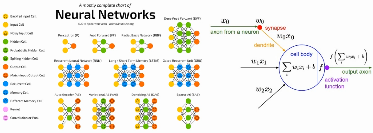

---

5. Chart

linear regressions + activation function 으로 하나의 logistic regression이 만들어지고,
이것이 하나의 Neural Net이 되어 다양한 모양의 Neural Network를 만들 수 있게 된다.

ex) RNN, LSTM, AE, SAE...

---

6. TensorBoard for XOR NN

TensorBoard : 모델링 과정에서 $w,b,loss$ 값들을 시각화 해 주는 도구

• https://hunkim.github.io/ml 참조

6-1. tensorboard 설치

# install
pip install tensorboard

# run
tensorboard --logdir=./logs/xor_logs    # tensorboard 저장 위치
# then open: http://127.0.0.1:6006      # ip와 포트번호를 통해 확인

---

6-2. Eager + TensorBoard (TF2 스타일)

# file: xor_tensorboard_tf2.py
import tensorflow as tf
import numpy as np

tf.random.set_seed(777)

# --- XOR toy data ---
x_data = np.array([[0, 0],
                   [0, 1],
                   [1, 0],
                   [1, 1]], dtype=np.float32)
y_data = np.array([[0],
                   [1],
                   [1],
                   [0]], dtype=np.float32)

# Dataset
dataset = tf.data.Dataset.from_tensor_slices((x_data, y_data)).batch(len(x_data))


def preprocess_data(features, labels):
    features = tf.cast(features, tf.float32)
    labels = tf.cast(labels, tf.float32)
    return features, labels


# --- Weights / Biases ---
W1 = tf.Variable(tf.random.normal([2, 10]), name="weight1")
b1 = tf.Variable(tf.random.normal([10]), name="bias1")

W2 = tf.Variable(tf.random.normal([10, 10]), name="weight2")
b2 = tf.Variable(tf.random.normal([10]), name="bias2")

W3 = tf.Variable(tf.random.normal([10, 10]), name="weight3")
b3 = tf.Variable(tf.random.normal([10]), name="bias3")

W4 = tf.Variable(tf.random.normal([10, 1]), name="weight4")
b4 = tf.Variable(tf.random.normal([1]), name="bias4")


def neural_net(features):
    layer1 = tf.sigmoid(tf.matmul(features, W1) + b1)
    layer2 = tf.sigmoid(tf.matmul(layer1, W2) + b2)
    layer3 = tf.sigmoid(tf.matmul(layer2, W3) + b3)
    hypothesis = tf.sigmoid(tf.matmul(layer3, W4) + b4)
    return layer1, layer2, layer3, hypothesis


def loss_fn(hypothesis, labels):
    # Binary cross-entropy
    cost = -tf.reduce_mean(
        labels * tf.math.log(hypothesis + 1e-7)
        + (1.0 - labels) * tf.math.log(1.0 - hypothesis + 1e-7)
    )
    return cost


optimizer = tf.keras.optimizers.SGD(learning_rate=0.1)

log_path = "./logs/xor_eager_tf2"
writer = tf.summary.create_file_writer(log_path)


def accuracy_fn(hypothesis, labels):
    predicted = tf.cast(hypothesis > 0.5, dtype=tf.float32)
    acc = tf.reduce_mean(tf.cast(tf.equal(predicted, labels), dtype=tf.float32))
    return acc


@tf.function
def train_step(features, labels, step):
    with tf.GradientTape() as tape:
        layer1, layer2, layer3, hypothesis = neural_net(features)
        loss_value = loss_fn(hypothesis, labels)

    grads = tape.gradient(
        loss_value,
        [W1, W2, W3, W4, b1, b2, b3, b4],
    )
    optimizer.apply_gradients(
        zip(grads, [W1, W2, W3, W4, b1, b2, b3, b4])
    )

    # TensorBoard summary
    with writer.as_default():
        tf.summary.scalar("loss", loss_value, step=step)
        tf.summary.histogram("weights1", W1, step=step)
        tf.summary.histogram("biases1", b1, step=step)
        tf.summary.histogram("layer1", layer1, step=step)
        tf.summary.histogram("weights2", W2, step=step)
        tf.summary.histogram("biases2", b2, step=step)
        tf.summary.histogram("layer2", layer2, step=step)
        tf.summary.histogram("weights3", W3, step=step)
        tf.summary.histogram("biases3", b3, step=step)
        tf.summary.histogram("layer3", layer3, step=step)
        tf.summary.histogram("weights4", W4, step=step)
        tf.summary.histogram("biases4", b4, step=step)
        tf.summary.histogram("hypothesis", hypothesis, step=step)

    return loss_value

EPOCHS = 3000
step = 0

for epoch in range(EPOCHS):
    for features, labels in dataset:
        features, labels = preprocess_data(features, labels)
        step += 1
        loss_value = train_step(features, labels, step)

    if epoch % 500 == 0:
        print(f"Epoch: {epoch}, Loss: {loss_value.numpy():.4f}")

# 평가
x_test = tf.cast(x_data, tf.float32)
y_test = tf.cast(y_data, tf.float32)
_, _, _, hypothesis = neural_net(x_test)
test_acc = accuracy_fn(hypothesis, y_test)
print(f"Testset Accuracy: {test_acc.numpy():.4f}")

print("Predictions:\n", tf.cast(hypothesis > 0.5, tf.int32).numpy())

# TensorBoard 실행 방법 (터미널):
#   tensorboard --logdir=./logs/xor_eager_tf2
# 브라우저에서 http://127.0.0.1:6006 접속

---

7. Keras Code (XOR)

import numpy as np
import tensorflow as tf

tf.random.set_seed(777)

x_data = np.array([[0, 0],
                   [0, 1],
                   [1, 0],
                   [1, 1]], dtype=np.float32)

y_data = np.array([[0],
                   [1],
                   [1],
                   [0]], dtype=np.float32)

model = tf.keras.models.Sequential([
    tf.keras.layers.Dense(10, input_dim=2, activation=tf.nn.sigmoid),
    tf.keras.layers.Dense(10, activation=tf.nn.sigmoid),
    tf.keras.layers.Dense(10, activation=tf.nn.sigmoid),
    tf.keras.layers.Dense(1,  activation=tf.nn.sigmoid),
])

model.compile(optimizer="adam",
              loss="binary_crossentropy",
              metrics=["binary_accuracy"])

tb_hist = tf.keras.callbacks.TensorBoard(
    log_dir="./logs/xor_logs_keras",
    histogram_freq=0,
    write_graph=True,
    write_images=True,
)

model.fit(x_data, y_data, epochs=5000, callbacks=[tb_hist], verbose=0)

pred = model.predict(x_data)
pred_label = (pred > 0.5).astype(np.int32)

print("Predicted probability:\n", pred)
print("Predicted label:\n", pred_label)

---

8. Summary

XOR 문제에서는 Logistic regression의 선형으로는 데이터를 구분할 수 없었다.
=> 따라서 Logistic regression을 쌓아서 2개의 Neural Net으로 만들고,
=> hidden layer를 추가한 Neural Network 구조로 XOR을 구분할 수 있게 되었다.

BackPropagation(연쇄법칙)을 통해,
각 노드의 $w,b$가 최종 출력과 cost에 어떤 영향을 주는지를 계산하고,
이 값을 이용해 gradient descent로 학습하게 된다.

TensorBoard를 사용하면,
학습 과정에서 $w,b,loss$가 어떻게 변하는지 시각적으로 확인할 수 있다.

---

모두를 위한 딥러닝 강좌 2
https://www.youtube.com/watch?v=7eldOrjQVi0&list=PLQ28Nx3M4Jrguyuwg4xe9d9t2XE639e5C