Lec-11 code 0 CNN basics Convolution / Pooling

remind

CNN (Convolutional Neural Network)

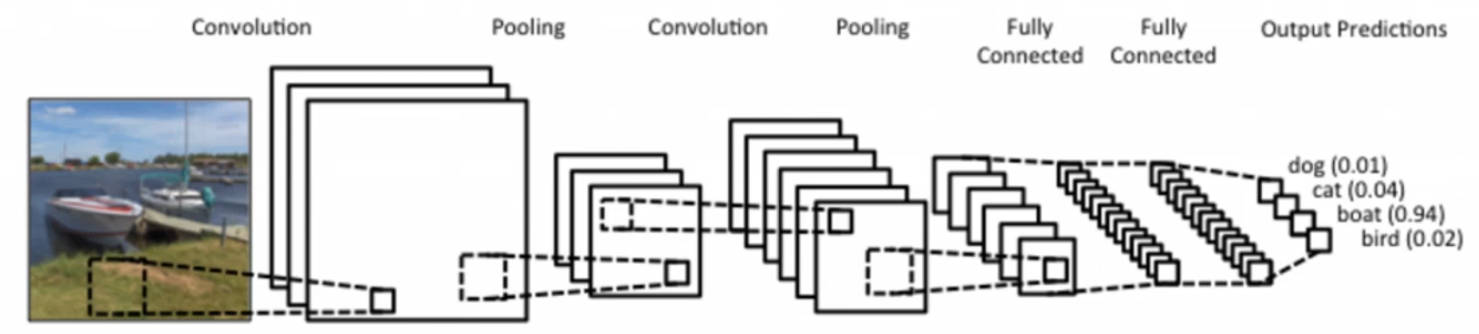
• 이미지 분류에서 가장 많이 쓰이는 방법.
• 일반적으로, convolution, pooling, fully connected 3개의 레이어로 구성된다.
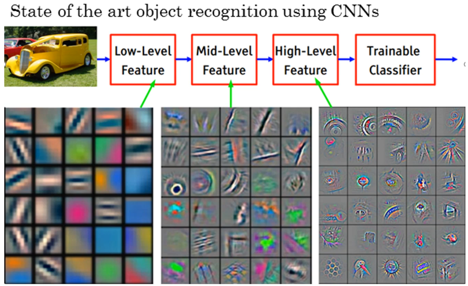
• 이때 convolution, pooling 레이어는 이미지의 모서리, 선, 질감, 모양, 부분 패턴 등 특징을 추출하는 레이어이다. → 즉, 이미지를 숫자로 된 의미 있는 특징 벡터로 변환한다.
• fully connected는 앞에서 뽑힌 특징 벡터를 받아서 어떤 클래스인지 결정하는 분류 레이어이다. → 특징을 각 클래스의 확률로 바꾼다.

---

2D Convolution Layer

Convolution Layer의 입력 예시

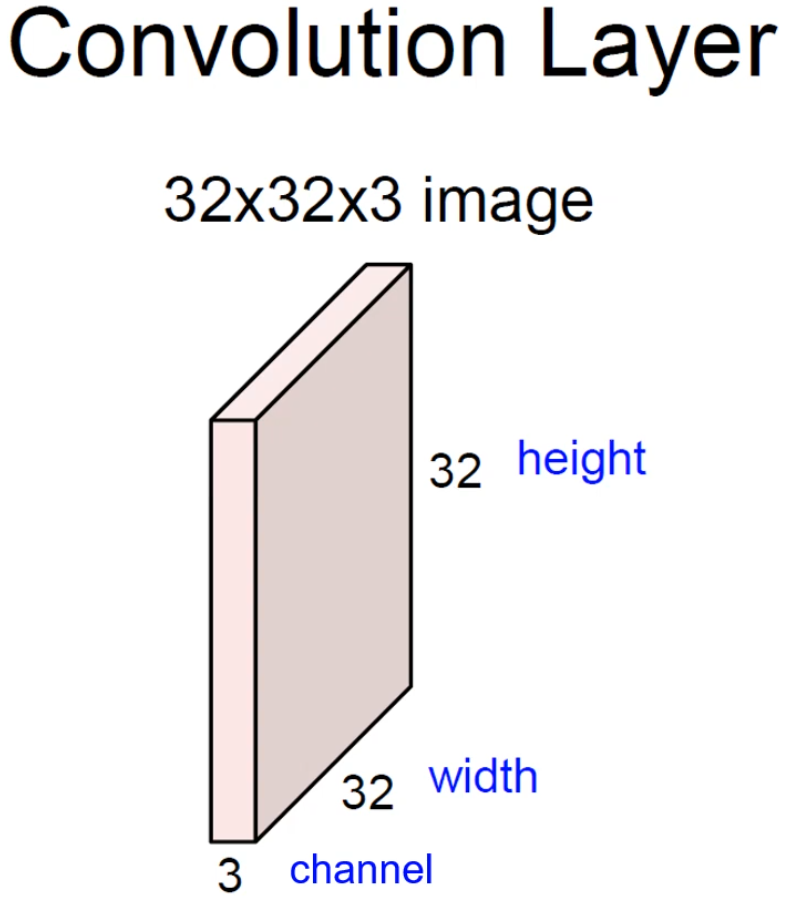
• 32×32×3 image : 일반적인 이미지가 입력으로 들어온 경우.

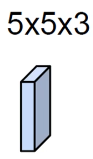
• 5×5×3 filter : 적당한 크기의 필터. 이때 채널의 크기는 항상 입력 채널의 크기와 같다.

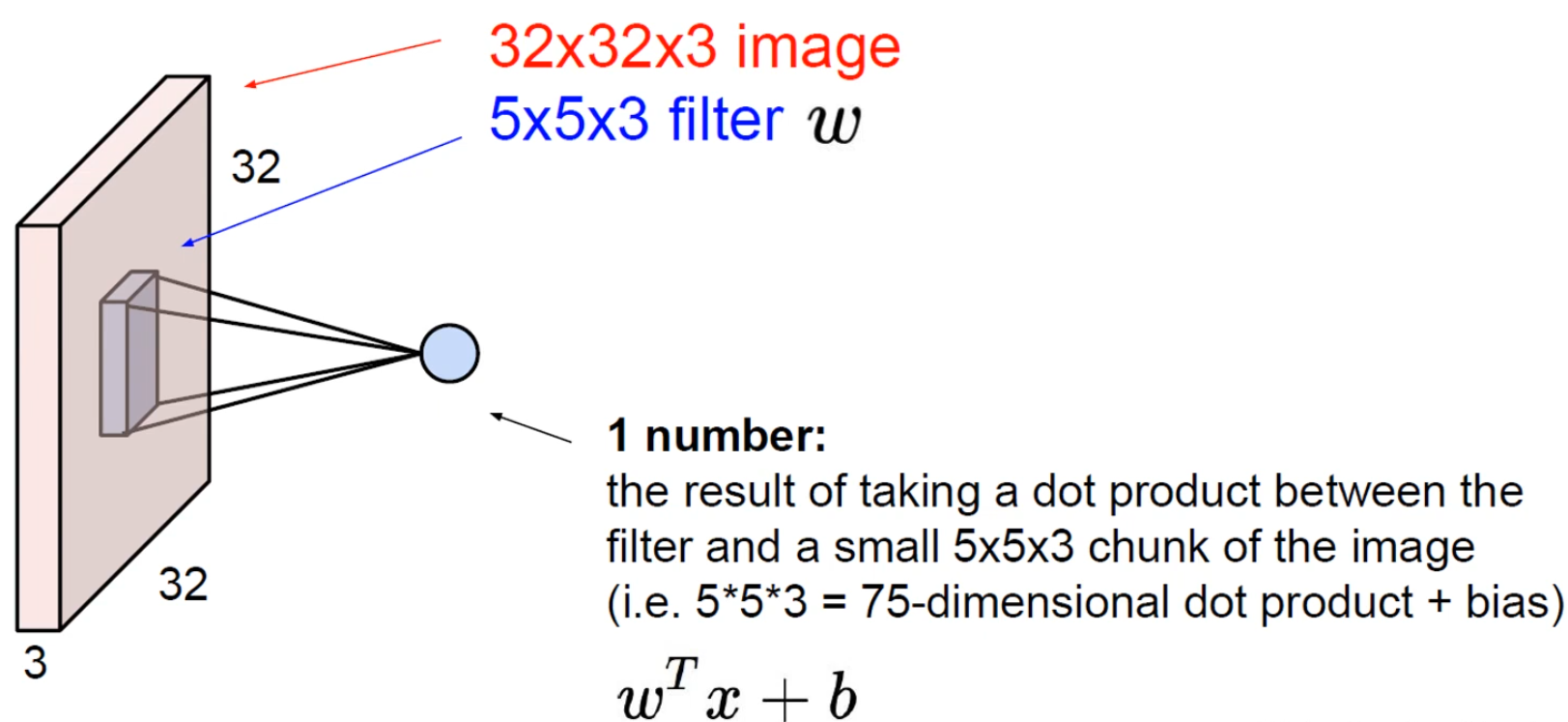
• 입력과 필터를 사용해 내적 연산을 진행하고, 1개의 숫자를 만들게 된다.

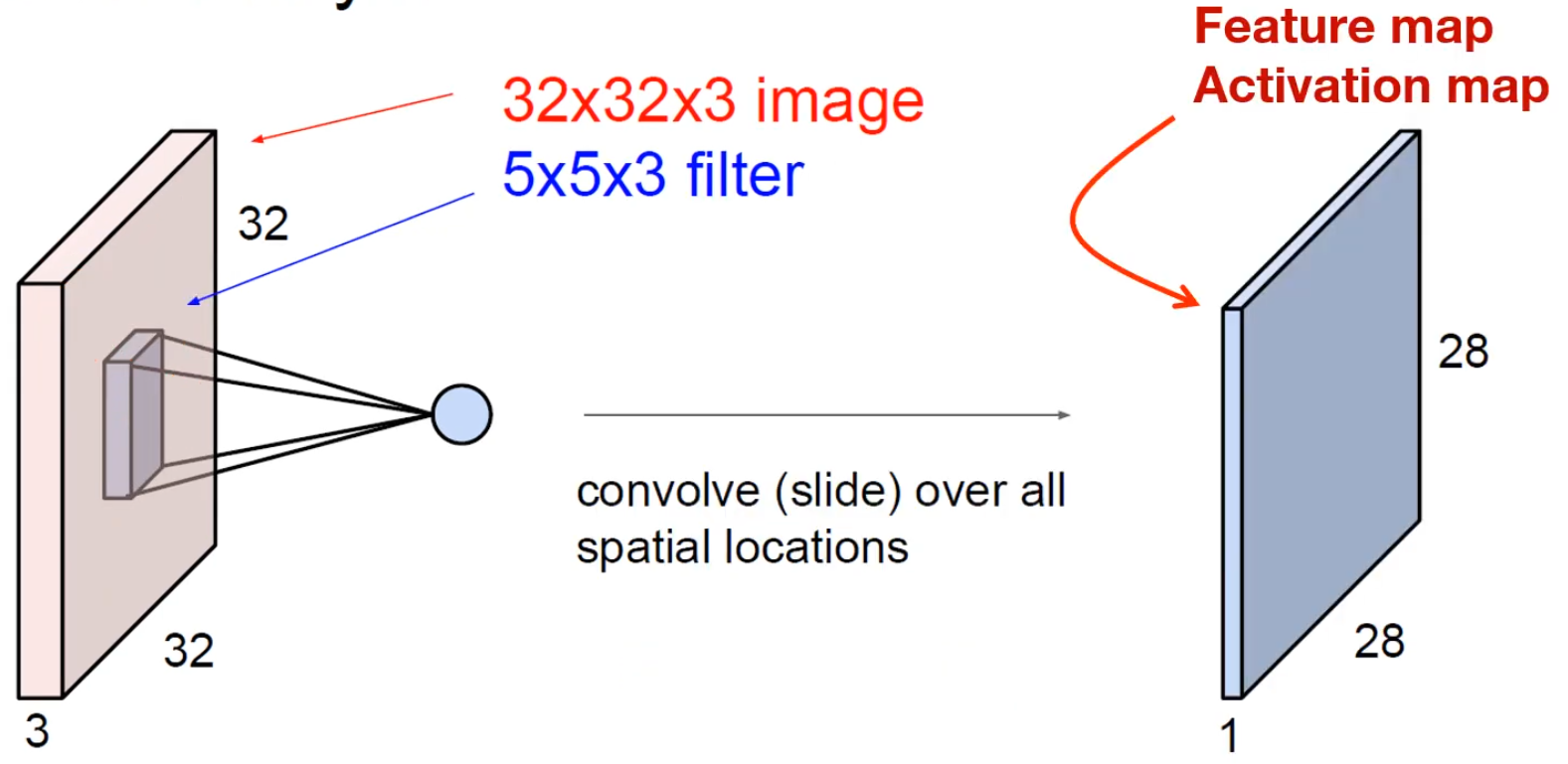
• 모든 연산을 종료하면 다음과 같은 output feature map 1장이 나오게 된다.

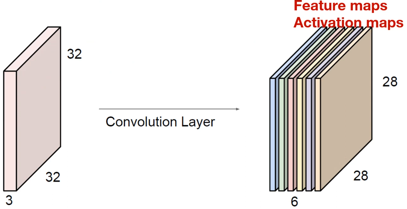
• filter 1개당 1개의 feature map이 나오므로, 6개의 필터를 사용하면 다음과 같이 채널이 6인 feature map이 생성되게 된다.

---

Computation

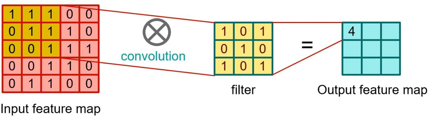
• input feature와 filter의 연산 과정이다. input과 filter의 동일한 위치의 값을 곱하고, 그 숫자들을 전부 더하여 1개의 숫자를 만들어낸다.

• 예시:

  $1\times1 + 1\times0 + 1\times1 + 0\times0 + 1\times1 + 1\times0 + 0\times1 + 0\times0 + 1\times1 = 4$
  $1\times1 + 1\times0 + 0\times1 + 1\times0 + 1\times1 + 1\times0 + 0\times1 + 1\times0 + 1\times1 = 3$
  $1\times1 + 0\times0 + 0\times1 + 1\times0 + 1\times1 + 0\times0 + 1\times1 + 1\times0 + 1\times1 = 4$
  ...

---

Multi Channel, Many filters

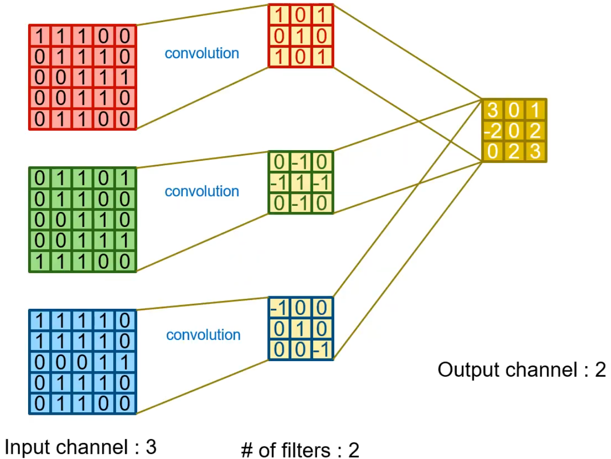
• RGB 하나의 이미지에 대해 2개의 필터를 사용했다.

---

4D Tensor

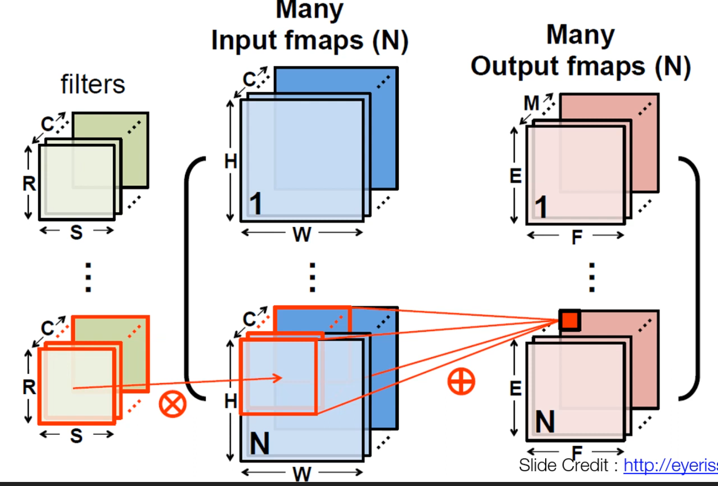
• 이 이미지와 같이 $N$개 filter에 대해 $N$개의 연산을 수행한다.

---

Activation Function

ReLU

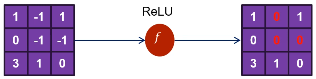
• 0보다 작은 값을 0으로 만든다.

---

Code 설명

tf.keras.layers.Conv2D 주요 인자

• filters
  정수. 출력 공간의 차원 수(즉, 컨볼루션의 출력 필터 개수).

• kernel_size
  정수 하나 또는 길이 2의 정수 튜플/리스트. 2D 컨볼루션 윈도의 높이와 너비를 지정. 하나의 정수로 주면 모든 공간 차원에 동일한 값을 사용.

• strides
  정수 하나 또는 길이 2의 정수 튜플/리스트. 높이와 너비 방향의 스트라이드를 지정한다. 하나의 정수로 주면 모든 공간 차원에 동일한 값을 사용한다.
  단, stride 값을 1이 아닌 값으로 지정하면, dilation_rate도 1이 아닌 값으로 지정하는 것과는 호환되지 않는다.

• padding
"valid" 또는 "same" 중 하나(대소문자 구분 없음).

• data_format
  문자열. "channels_last"(기본값) 또는 "channels_first". 입력 차원 순서를 결정한다.

  • channels_last → 입력 형태: (batch, height, width, channels)
  • channels_first → 입력 형태: (batch, channels, height, width)
    기본값은 사용자 Keras 설정 파일(~/.keras/keras.json)의 image_data_format 값을 따르고, 설정한 적이 없다면 기본은 "channels_last"이다.

• activation
  사용할 활성화 함수. 아무것도 지정하지 않으면 활성화를 적용하지 않으며(즉, 선형 활성화), $a(x)=x$이다.

• use_bias
  레이어가 바이어스 벡터를 사용할지 여부를 나타내는 불리언이다.

• kernel_initializer
  커널 가중치 행렬을 위한 이니셜라이저이다.

• bias_initializer
  바이어스 벡터를 위한 이니셜라이저이다.

• kernel_regularizer
  커널 가중치 행렬에 적용되는 정규화 함수이다.

• bias_regularizer
  바이어스 벡터에 적용되는 정규화 함수이다.

---

padding 정리

구분	Valid	Same
Value	$P = 0$	$P_{\text{start}} = \left\lceil \dfrac{S\left\lceil \dfrac{I}{S} \right\rceil - I + F - S}{2} \right\rceil$ $P_{\text{end}} = \left\lfloor \dfrac{S\left\lceil \dfrac{I}{S} \right\rceil - I + F - S}{2} \right\rfloor$
Illustration	패딩 없이 커널이 입력 내부만 스캔	위아래·좌우에 패딩을 추가해 출력 특성맵의 공간 크기가 $\left\lceil \dfrac{I}{S} \right\rceil$이 되도록 맞춤
Purpose	• 패딩이 없음 • 크기가 딱 나누어떨어지지 않으면 마지막 위치의 컨볼루션이 생략됨	• 출력 크기를 수식적으로 다루기 편하도록 패딩 추가 • 흔히 ‘half padding’이라고도 부름

---

Code

1) import

import numpy as np
import tensorflow as tf
from tensorflow import keras
import matplotlib.pyplot as plt

print(tf.__version__)
print(keras.__version__)

tf.enable_eager_execution()

---

2) toy image

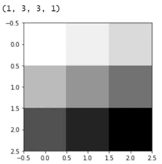
image = tf.constant(
    [
        [[1], [2], [3]],
        [[4], [5], [6]],
        [[7], [8], [9]],
    ],
    dtype=np.float32,
)

print(image.shape)

plt.imshow(image.numpy().reshape(3, 3), cmap="Greys")
plt.show()

---

3) Simple convolution Layer – No Padding

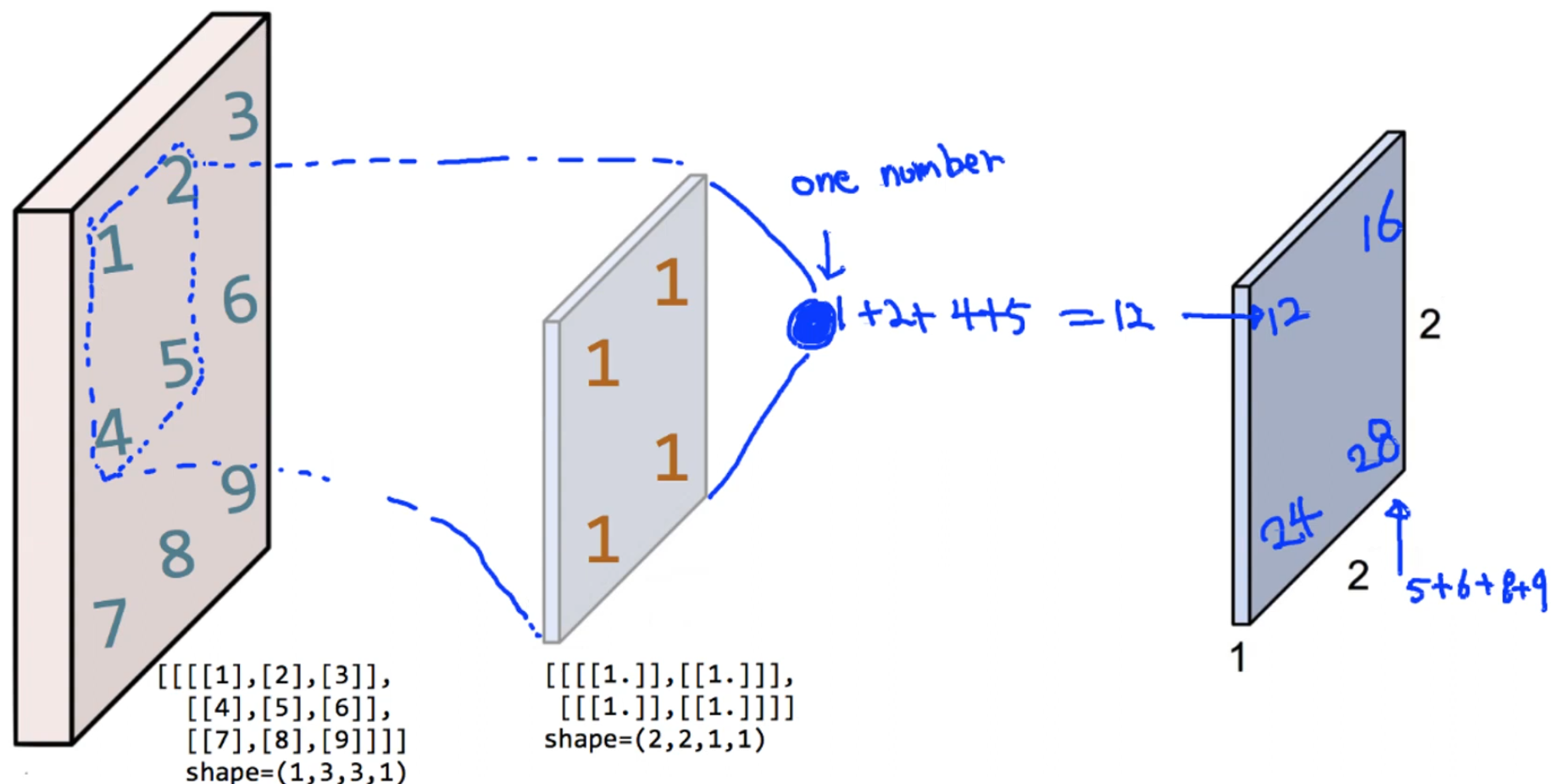
print("image.shape", image.shape)

weight = np.array(
    [
        [[[1.]], [[1.]]],
        [[[1.]], [[1.]]],
    ]
)
print("weight.shape", weight.shape)

weight_init = tf.constant_initializer(weight)

conv2d = keras.layers.Conv2D(
    filters=1,
    kernel_size=2,
    padding="VALID",
    kernel_initializer=weight_init,
)(image)

print("conv2d.shape", conv2d.shape)
print(conv2d.numpy().reshape(2, 2))

plt.imshow(conv2d.numpy().reshape(2, 2), cmap="gray")
plt.show()

---

4) Simple convolution Layer – add Padding

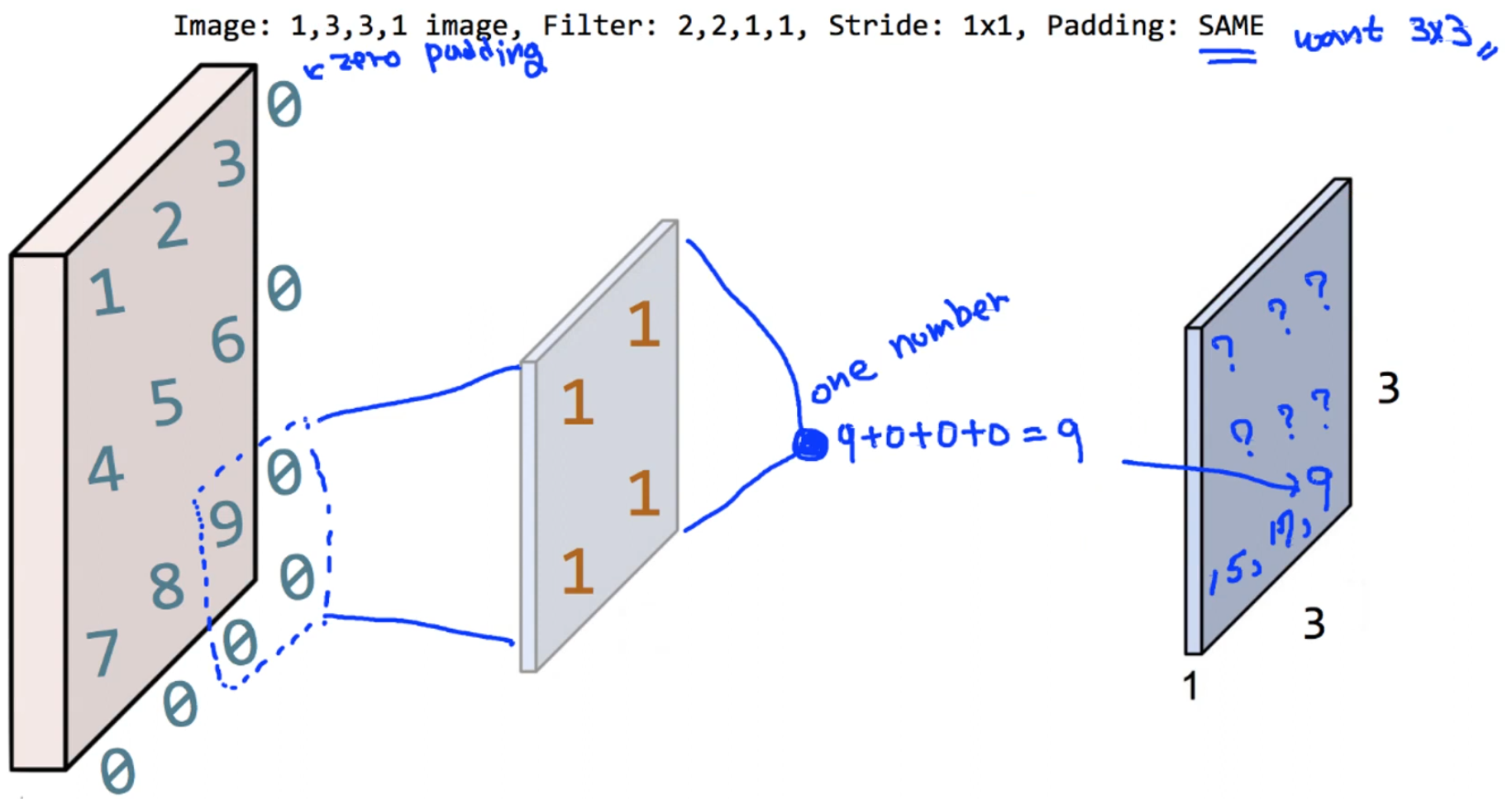
print("image.shape", image.shape)

weight = np.array(
    [
        [[[1.]], [[1.]]],
        [[[1.]], [[1.]]],
    ]
)
print("weight.shape", weight.shape)

weight_init = tf.constant_initializer(weight)

conv2d = keras.layers.Conv2D(
    filters=1,
    kernel_size=2,
    padding="SAME",
    kernel_initializer=weight_init,
)(image)

print("conv2d.shape", conv2d.shape)
print(conv2d.numpy().reshape(3, 3))

plt.imshow(conv2d.numpy().reshape(3, 3), cmap="gray")
plt.show()

---

5) 3 Filters

print("image.shape", image.shape)

weight = np.array(
    [
        [[[1., 10., -1.]], [[1., 10., -1.]]],
        [[[1., 10., -1.]], [[1., 10., -1.]]],
    ]
)
print("weight.shape", weight.shape)

weight_init = tf.constant_initializer(weight)

conv2d = keras.layers.Conv2D(
    filters=3,
    kernel_size=2,
    padding="SAME",
    kernel_initializer=weight_init,
)(image)

print("conv2d.shape", conv2d.shape)

feature_maps = np.swapaxes(conv2d.numpy(), 0, 3)

for i, feature_map in enumerate(feature_maps):
    print(feature_map.reshape(3, 3))
    plt.subplot(1, 3, i + 1)
    plt.imshow(feature_map.reshape(3, 3), cmap="gray")

plt.show()

---

Pooling

1. Max Pooling
   필터의 범위 안에서 가장 큰 숫자를 선택한다.
   ⇒ 중요한 정보를 뽑아서 사이즈를 줄였으므로 Sub Sampling이라고도 부른다.
   ⇒ 주로 이 max pooling을 많이 쓰는데, 이는 숫자가 클수록 convolution 필터가 찾고자 했던 특징과 더 잘 맞기 때문이다.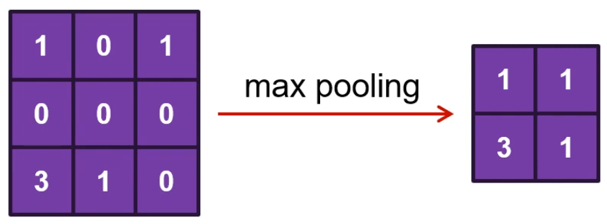

   

2. Average Pooling
   필터의 범위 안 숫자의 평균을 가진다.

---

code

1) tf.keras.layers.MaxPool2D

__init__(
    pool_size=(2, 2),
    strides=None,
    padding="valid",
    data_format=None,
    **kwargs
)

---

2) Max Pooling

image = tf.constant(
    [
        [
            [[4], [3]],
            [[2], [1]],
        ]
    ],
    dtype=np.float32,
)

pool = keras.layers.MaxPool2D(
    pool_size=(2, 2),
    strides=1,
    padding="VALID",
)(image)
# padding을 "SAME"으로 바꾸면 처음 입력과 같은 크기의 결과가 나온다.
# pool = keras.layers.MaxPool2D(pool_size=(2, 2), strides=1, padding="SAME")(image)

print(pool.shape)
print(pool.numpy())

---

3) loading MNIST data

mnist = keras.datasets.mnist
class_names = ["0", "1", "2", "3", "4", "5", "6", "7", "8", "9"]

(train_images, train_labels), (test_images, test_labels) = mnist.load_data()

train_images = train_images.astype(np.float32) / 255.0
test_images = test_images.astype(np.float32) / 255.0

img = train_images[0]
plt.imshow(img, cmap="gray")
plt.show()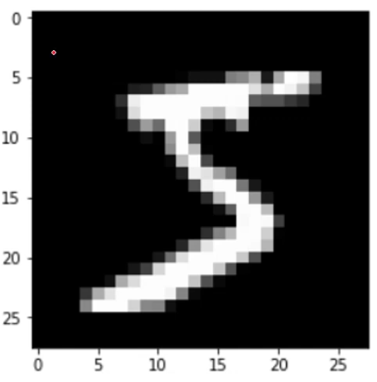

---

4) Convolution Layer

img = img.reshape(-1, 28, 28, 1)
# img는 numpy array로 반환되기 때문에 tensor로 변환해야 한다.
img = tf.convert_to_tensor(img)

weight_init = keras.initializers.RandomNormal(stddev=0.01)

conv2d = keras.layers.Conv2D(
    filters=5,
    kernel_size=3,
    strides=(2, 2),
    padding="SAME",
    kernel_initializer=weight_init,
)(img)

print(conv2d.shape)

feature_maps = np.swapaxes(conv2d.numpy(), 0, 3)
for i, feature_map in enumerate(feature_maps):
    plt.subplot(1, 5, i + 1)
    plt.imshow(feature_map.reshape(14, 14), cmap="gray")

plt.show()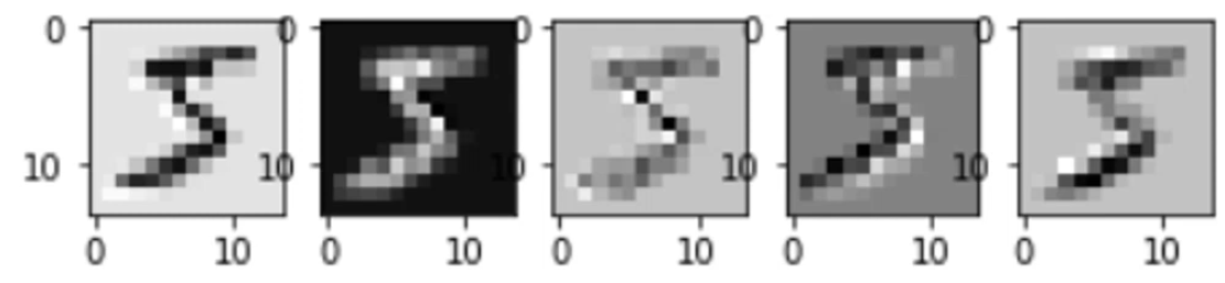

---

5) Pooling Layer

pool = keras.layers.MaxPool2D(
    pool_size=(2, 2),
    strides=(2, 2),
    padding="SAME",
)(conv2d)

print(pool.shape)

feature_maps = np.swapaxes(pool.numpy(), 0, 3)
for i, feature_map in enumerate(feature_maps):
    plt.subplot(1, 5, i + 1)
    plt.imshow(feature_map.reshape(7, 7), cmap="gray")

plt.show()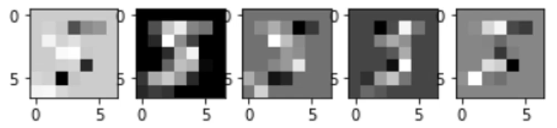

---

6) Fully Connected Layer

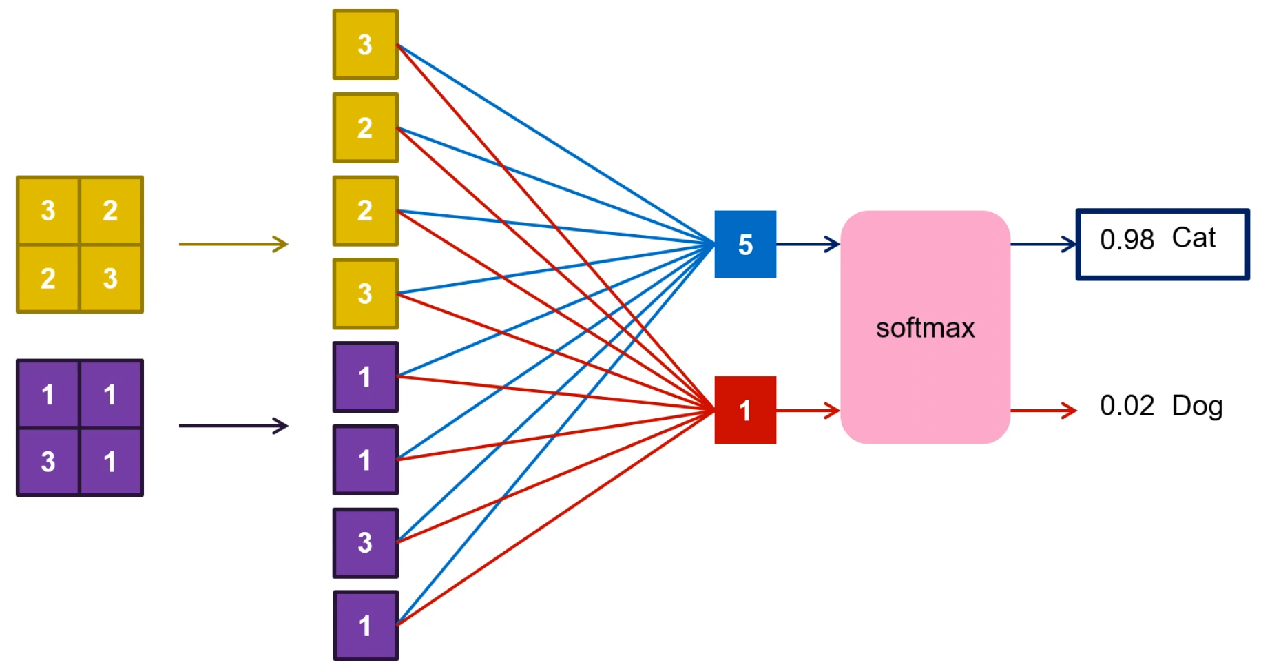
⇒ pooling 된 결과를 벡터 형태로 쭉 펴준 뒤, 전부 연결해서 FC로 만든다.

---

정리

CNN은 convolution layer, pooling layer를 통해 feature를 뽑아내는 feature extraction 역할을 하고 마지막에 fully connected에서 실제 classification 하는 역할을 한다.

---

출처: 모두를 위한 딥러닝 강좌 2
https://www.youtube.com/watch?v=7eldOrjQVi0&list=PLQ28Nx3M4Jrguyuwg4xe9d9t2XE639e5C