★ DataFrame (2D)
✓ 2차원의 labeled data structure with columns of potentially different types이다.
✓ index = row labels / columns = column labels
✓ Kinds of input Data type
◼︎Dict of 1D ndarrays,lists,dicts,Series
◼︎2D numpy.ndarray
◼︎Structured or record ndarray
◼︎A Series
◼︎Another DataFrame)
▼ 구성 방법 예시 ▼ (data type별)
1. From dict of Series or dicts 구성 예시
>>> d = {
	"one" = pd.Series([1.0, 2.0, 3.0], index=["a", "b", "c"]),
    "two" = pd.Series([1.0, 2.0, 3.0, 4.0], index=["a", "b", "c", "d"]),
}
>>> df = pd.DataFrame(d)
>>> df
>>>
	one	two
a	1.0	1.0
b	2.0	2.0
c	3.0	3.0
d	NaN	4.0
>>> df.index
>>> Index(['a','b','c','d'],dtype='object')
>>> df.columns
>>> Index(['one','two'],dtype='object')
# When a particular set of columns is passed along with a dict of data,
the passed columns override the keys in the dict
2. From dict of ndarrays / lists
✓ The ndarrrays must all be the same length.
>>> d = {"one": [1.0, 2.0, 3.0, 4.0], "two": [4.0, 3.0, 2.0, 1.0]}
>>> pd.DataFrame(d)
>>>
	one	two
a	1.0	4.0
b	2.0	3.0
c	3.0	2.0
d	4.0	1.0
3. Frome structured or record array
✓ DataFrame이 2D NumPy ndarrray처럼 정확히 work 안함
>>> data = np.zeros((2,), dtype=[("A", "i4"), ("B", "f4"), ("C", "a10")]) # 이 부분 체크 필요
>>> data[:] = [(1, 2.0, "Hello"), (2, 3.0, "World")]
>>> pd.DataFrame(data)
>>>
	A	B	C
0	1	2.0	b'Hello'
1	2	3.0	b'World'
>>> pd.DataFrame(data, index=["first", "second"])
	A	B	C
first	1	2.0	b'Hello'
second	2	3.0	b'World'
>>> pd.DataFrame(data, columns=["C", "A", "B"]) # column name 바꾸는거
	C		A	B
0	b'Hello'	1	2.0
1	b'World'	2	3.0
4. From a list of dicts
>>> data2 = [{"a": 1, "b": 2}, {"a": 5, "b": 10, "c": 20}]
>>> pd.DataFrame(data2)
>>>
	a	b	c
0	1	2	NaN
1	5	10	20.0
5. From a dict of tuples
✓ 이게 잘 활용되는 예를 찾아봐야 할 듯???
>>> pd.DataFrame(
	{
    	("a","b"): {("A","B"):1, ("A","C"):2},
        ("a","a"): {("A","C"):3, ("A","B"):4},
        ("a","c"): {("A","B"):5, ("A","C"):6},
        ("b","a"): {("A","C"):7, ("A","B"):8},
        ("b","b"): {("A","D"):9, ("A","B"):10},
    }
)
>>>
		a			b
        	b	a	c	a	b
A	B	1.0	4.0	5.0	8.0	10.0
	C	2.0	3.0	6.0	7.0	NaN
    	D	NaN	NaN	NaN	NaN	9.0
6. From a Series
✓ The result will be a DataFame (same index as the input Series, one column whose name is the original name of the Series)
7. From a list of namedtuples
✓ namedtuple의 field names가 DataFrame의 columns를 결정한다.
✓ namedtuple 특성 파악 필요
>>> from collections import namedtuple
>>> Point = namedtuple("Point", "x y")
>>> pd.DataFrame([Point(0,0), Point(0,3), (2,3)])
>>>
	x	y
0	0	0
1	0	3
2	2	3
>>> Point3D = namedtuple("Point3D", "x y z")
>>> pd.DataFrame([Point3D(0, 0, 0), Point3D(0, 3, 5), Point(2, 3)])
>>>
	x	y	z
0	0	0	0.0
1	0	3	5.0
2	2	3	NaN
8. From a list of dataclasses
✓ Data Classes 의 list를 passing하는 것 (list of dictionaries를 passing하는 것과 같다)
✓ 다만 all values가 dataclasses여야하고 mixing types이면 TypeError뜸.
>>> from dataclasses import make_dataclass
>>> Point = make_dataclass("Point", [("x", int), ("y", int)])
>>> pd.DataFrame([Point(0, 0), Point(0, 3), Point(2, 3)])
>>>
	x	y
0	0	0
1	0	3
2	2	3
000. Missing data
✓ pandas에서 missing values를 어떻게 다루는지...(정리 예정)
https://pandas.pydata.org/docs/user_guide/missing_data.html#missing-data
▼ Alternate constructors ▼
1. DataFrame.from_dict
✓ dict of dicts / array-like sequences를 가지고 DataFrame을 return함
>>> pd.DataFrame.from_dict(dict([("A", [1, 2, 3]), ("B", [4, 5, 6])]))
>>>
	A	B
0	1	4
1	2	5
2	3	6
# default로 dict의 key가 columns로 받아짐
# orient='index'로 하면 key가 row labels로 받아짐
>>> pd.DataFrame.from_dict(
	dict([("A", [1, 2, 3]), ("B", [4, 5, 6])]),
    orient="index",
    columns=["one","two","three"],
)
>>>
	one	two	three
A	1	2	3
B	4	5	6
2. DataFrame.from_records
✓ list of tuples / ndarray with structured dtype을 가지고 DataFrame 구성
✓ 일반적으로 DataFrame 구성하지만 specific field를 index로 할 수 있다
>>> data
>>> array([(1, 2., b'Hello'), (2, 3., b'World')], dtype=[('A', '<i4'), ('B', '<f4'), ('C', 'S10')])
>>> pd.DataFrame.from_records(data, index="C")
>>>
		A	B
C
b'Hello'	1	2.0
b'World'	2	3.0
▼ Handlings ▼
Column selection, addition, deletion
# getting, setting, deleting
>>> df["one"]
>>>
a	1.0
b	2.0
c	3.0
d	NaN
>>> df["three"] = df["one"] * df["two"]
>>> df["flag"] = df["one"] > 2
>>> df
>>>
	one	two	three	flag
a	1.0	1.0	1.0	False
b	2.0	2.0	4.0	False
c	3.0	3.0	9.0	True
d	NaN	4.0	NaN	False
# delete / pop
>>> del df["two"]
>>> three = df.pop("three")
>>> df
>>>
	one	flag
a	1.0	False
b	2.0	False
c	3.0	True
d	NaN	False
>>> df["foo"] = "bar" # insert scalar value
>>>	df
>>>
	one	flag	foo
a	1.0	False	bar
b	2.0	False	bar
c	3.0	True	bar
d	NaN	False	bar
>>> df["one_trunc"] = df["one"][:2] # insert a Series
>>> df
>>>
	one flag	foo	one_trunc
a	1.0	False	bar	1.0
b	2.0	False	bar	2.0
c	3.0	True	bar	NaN
d	NaN	False	bar	NaN
# insert raw ndarray (length는 같아야 함)
>>> df.insert(1, "bar", df["one"])
>>> df
>>>
	one bar	flag	foo	one_trunc
a	1.0	1.0	False	bar	1.0
b	2.0	2.0	False	bar	2.0
c	3.0	3.0	True	bar	NaN
d	NaN	NaN	False	bar	NaN
Assigning new columns in method chains
✓ assign always returns a copy of the data, leaving the original DataFrrame untouched
✓ 보완 필요...
>>> iris = pd.read_csv("data/iris.data")
>>> iris.head()
>>>
SepalLength SepalWidth PetalLength PetalWidth Name
0 5.1 3.5 1.4 0.2 Iris-setosa
1 4.9 3.0 1.4 0.2 Iris-setosa
2 4.7 3.2 1.3 0.2 Iris-setosa
3 4.6 3.1 1.5 0.2 Iris-setosa
4 5.0 3.6 1.4 0.2 Iris-setosa
>>> iris.assign(sepal_ratio=iris["SepalWidth"] / iris["SepalLength"]).head()
>>>
SepalLength SepalWidth PetalLength PetalWidth Name sepal_ratio
0 5.1 3.5 1.4 0.2 Iris-setosa 0.686275
1 4.9 3.0 1.4 0.2 Iris-setosa 0.612245
2 4.7 3.2 1.3 0.2 Iris-setosa 0.680851
3 4.6 3.1 1.5 0.2 Iris-setosa 0.673913
4 5.0 3.6 1.4 0.2 Iris-setosa 0.720000
>>> iris.assign(sepal_ratio=lambda x: (x["SepalWidth"] / x["SepalLength"])).head()
>>> # output 위와 같다
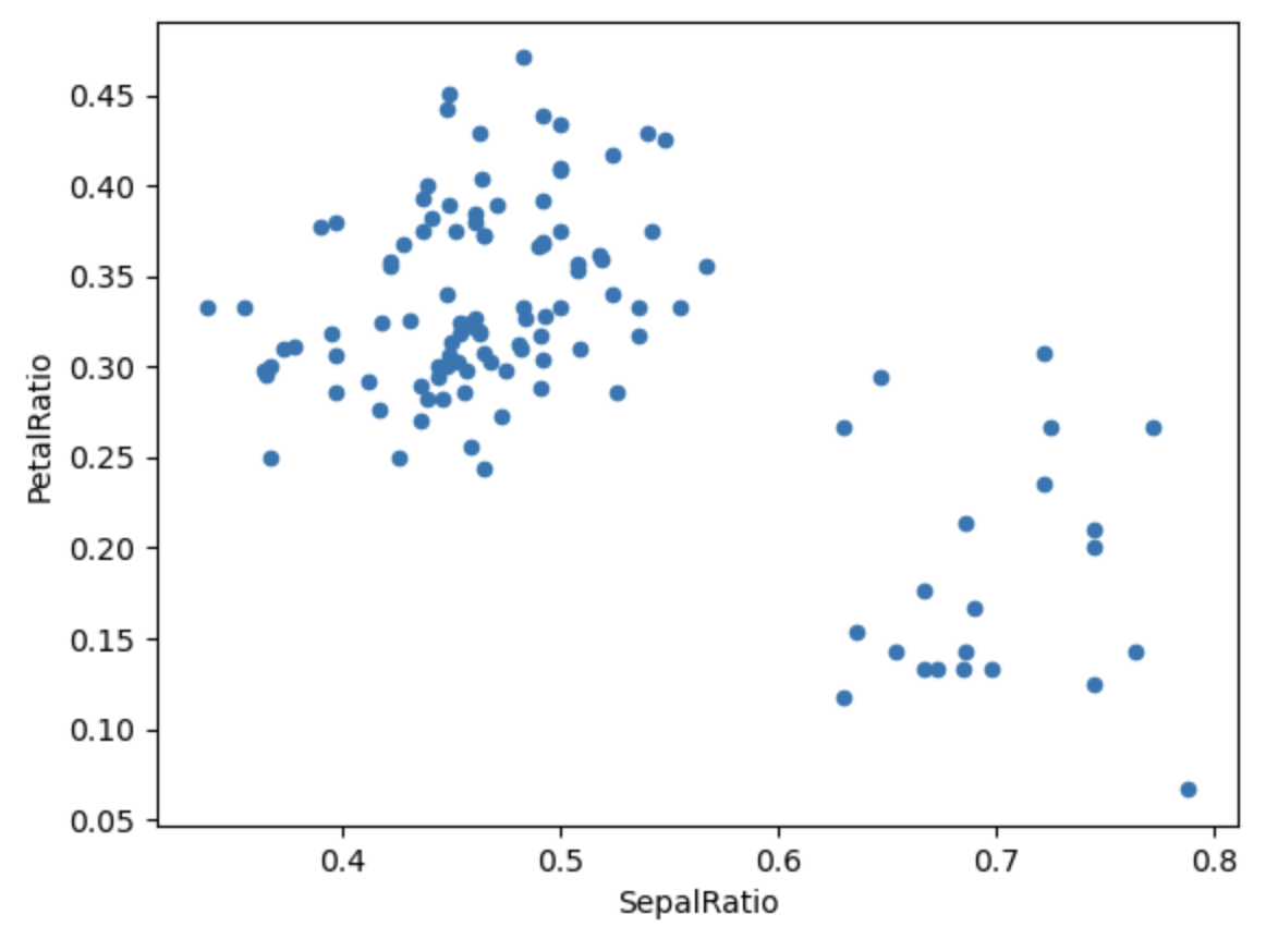
>>> (
iris.query("SepalLength > 5")
.assign(
SepalRatio=lambda x: x.SepalWidth / x.SepalLength,
PetalRatio=lambda x: x.PetalWidth / x.PetalLength,
)
.plot(kind="scatter", x="SepalRatio", y="PetalRatio")
)
>>> dfa = pd.DataFrame({"A": [1, 2, 3], "B": [4, 5, 6]})
>>> dfa.assign(C=lambda x: x["A"] + x["B"], D=lambda x: x["A"] + x["C"])
>>>
A B C D
0 1 4 5 6
1 2 5 7 9
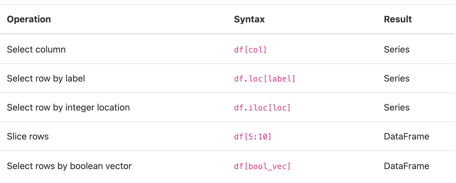
2 3 6 9 12Indexing / selection
참고(추가 예정)
Indexing : https://pandas.pydata.org/docs/user_guide/indexing.html#indexing
Reindexing : https://pandas.pydata.org/docs/user_guide/basics.html#basics-reindexing
Data alignment and arithmetic
✓ DataFrame object들 사이의 alignment에서 보면, union of column and index로 결과가 구해짐
✓ DataFrame 과 Series 사이의 alignment에서 보면, DataFrame의 columns에 Series의 index가 정렬되고 이것이 row 방향으로 broadcasting 되며 결과 구해짐
>>> df = pd.DataFrame(np.random.randn(10, 4), columns=["A", "B", "C", "D"])
>>> df2 = pd.DataFrame(np.random.randn(7, 3), columns=["A", "B", "C"])
>>> df + df2
>>> # index와 column에 맞춰 연산
	A		B		C		D
0	0.045691	-0.014138	1.380871	NaN
1	-0.955398	-1.501007	0.037181	NaN
2	-0.662690 	1.534833	-0.859691	NaN
3	-2.452949 	1.237274	-0.133712	NaN
4 	1.414490 	1.951676	-2.320422	NaN
5	-0.494922	-1.649727	-1.084601	NaN
6	-1.047551	-0.748572	-0.805479	NaN
7	NaN		NaN		NaN		NaN
8	NaN		NaN		NaN		NaN
9	NaN		NaN		NaN		NaN
>>> df - df.iloc[0]
>>> # Series가 broadcasting 되면서 연산
	A		B		C		D
0	0.000000	0.000000	0.000000	0.000000
1	-1.359261	-0.248717	-0.453372	-1.754659
2	0.253128	0.829678	0.010026	-1.991234
3	-1.311128	0.054325	-1.724913	-1.620544
4	0.573025	1.500742	-0.676070	1.367331
5	-1.741248	0.781993	-1.241620	-2.053136
6	-1.240774	-0.869551	-0.153282	0.000430
7	-0.743894	0.411013	-0.929563	-0.282386
8	-1.194921	1.320690	0.238224	-1.482644
9	2.293786	1.856228	0.773289	-1.446531
# scalars로 연산 될 때
>>> df * 5 + 2
>>> 1 / df
>>> df ** 4
# Boolean로 연산 될 때
>>> df1 = pd.DataFrame({"a": [1, 0, 1], "b": [0, 1, 1]}, dtype=bool)
>>> df2 = pd.DataFrame({"a": [0, 1, 1], "b": [1, 1, 0]}, dtype=bool)
>>> df1 & df2
>>>
	a	b
0	False	False
1	False	True
2	True	False
>>> df1 | df2
>>> df1 ^ df2
>>> -df1
참고(추가 예정)
Broadcasting : https://numpy.org/doc/stable/user/basics.broadcasting.html
Flexible binary operations : https://pandas.pydata.org/docs/user_guide/basics.html#basics-binop
Transposing
✓ transpose하는 것은 'T'를 사용하면 된다(ndarray와 비슷하게)
>>> df[:5].T
>>>
	0		1		2		3		4
A	0.271860	-1.087401	0.524988	-1.039268 	0.844885
B	-0.424972	-0.673690 	0.404705	-0.370647 	1.075770
C	0.567020	0.113648 	0.577046	-1.157892	-0.109050
D	0.276232	-1.478427	-1.715002	-1.344312 	1.643563
DataFrame interoperability with NumPy functions
✓ Elementwise로 연산되는 NumPy functions(log, exp, sqrt ...)는 Series와 DataFrame에서 사용 가능하다
✓ DataFrame은 ndarray와 같이 적용하기 어렵지만, Series 같은 경우에는 NumPy's universal functions를 적용할 수 있다.
>>> np.exp(df)
>>> np.asarray(df)
>>>
array([[ 0.2719, -0.425 ,  0.567 ,  0.2762],
       [-1.0874, -0.6737,  0.1136, -1.4784],
       [ 0.525 ,  0.4047,  0.577 , -1.715 ],
       [-1.0393, -0.3706, -1.1579, -1.3443],
       [ 0.8449,  1.0758, -0.109 ,  1.6436],
       [-1.4694,  0.357 , -0.6746, -1.7769],
       [-0.9689, -1.2945,  0.4137,  0.2767],
       [-0.472 , -0.014 , -0.3625, -0.0062],
       [-0.9231,  0.8957,  0.8052, -1.2064],
       [ 2.5656,  1.4313,  1.3403, -1.1703]])
>>> ser = pd.Series([1, 2, 3, 4])
>>>
0     2.718282
1     7.389056
2    20.085537
3    54.598150
# index 순서 달라도 가능 (label별로 자동 정렬)
>>> ser1 = pd.Series([1, 2, 3], index=["a", "b", "c"])
>>> ser2 = pd.Series([1, 3, 5], index=["b", "a", "c"])
>>> np.remainder(ser1, ser2)
>>>
a	1
b	0
c	3
>>> ser3 = pd.Series([2, 4, 6], index=["b", "c", "d"])
# index 다른 것은 missing value
>>> np.remainder(ser1, ser3)
>>>
a	NaN
b	0.0
c	3.0
d	NaN
#
>>>
# Series와 Index에 binary ufunc 적용되면, 우선적으로 Series로 return함
>>> ser = pd.Series([1, 2, 3])
>>> idx = pd.Index([4, 5, 6])
>>> np.maximum(ser, idx)
>>>
0	4
1	5
2	6
Console display
✓ DataFrame이 너무 클 때 console에 잘려서 display될 수 있다.
>>> baseball = pd.read_csv("data/baseball.csv") # dataset from plyr R package
>>> print(baseball)
>>>
       id     player  year  stint team  lg   g   ab   r    h  X2b  X3b  hr   rbi   sb   cs  bb    so  ibb  hbp   sh   sf  gidp
0   88641  womacto01  2006      2  CHN  NL  19   50   6   14    1    0   1   2.0  1.0  1.0   4   4.0  0.0  0.0  3.0  0.0   0.0
1   88643  schilcu01  2006      1  BOS  AL  31    2   0    1    0    0   0   0.0  0.0  0.0   0   1.0  0.0  0.0  0.0  0.0   0.0
..    ...        ...   ...    ...  ...  ..  ..  ...  ..  ...  ...  ...  ..   ...  ...  ...  ..   ...  ...  ...  ...  ...   ...
98  89533   aloumo01  2007      1  NYN  NL  87  328  51  112   19    1  13  49.0  3.0  0.0  27  30.0  5.0  2.0  0.0  3.0  13.0
99  89534  alomasa02  2007      1  NYN  NL   8   22   1    3    1    0   0   0.0  0.0  0.0   0   3.0  0.0  0.0  0.0  0.0   0.0

[100 rows x 23 columns]

# to_string으로 tabular form으로 representation할 수 있음(단,console width랑 안 맞을 수도)
>>> print(baseball.iloc[-20:, :12].to_string())
>>>
       id     player  year  stint team  lg    g   ab   r    h  X2b  X3b
80  89474  finlest01  2007      1  COL  NL   43   94   9   17    3    0
81  89480  embreal01  2007      1  OAK  AL    4    0   0    0    0    0
82  89481  edmonji01  2007      1  SLN  NL  117  365  39   92   15    2
83  89482  easleda01  2007      1  NYN  NL   76  193  24   54    6    0
84  89489  delgaca01  2007      1  NYN  NL  139  538  71  139   30    0
85  89493  cormirh01  2007      1  CIN  NL    6    0   0    0    0    0
86  89494  coninje01  2007      2  NYN  NL   21   41   2    8    2    0
87  89495  coninje01  2007      1  CIN  NL   80  215  23   57   11    1
88  89497  clemero02  2007      1  NYA  AL    2    2   0    1    0    0
89  89498  claytro01  2007      2  BOS  AL    8    6   1    0    0    0
90  89499  claytro01  2007      1  TOR  AL   69  189  23   48   14    0
91  89501  cirilje01  2007      2  ARI  NL   28   40   6    8    4    0
92  89502  cirilje01  2007      1  MIN  AL   50  153  18   40    9    2
93  89521  bondsba01  2007      1  SFN  NL  126  340  75   94   14    0
94  89523  biggicr01  2007      1  HOU  NL  141  517  68  130   31    3
95  89525  benitar01  2007      2  FLO  NL   34    0   0    0    0    0
96  89526  benitar01  2007      1  SFN  NL   19    0   0    0    0    0
97  89530  ausmubr01  2007      1  HOU  NL  117  349  38   82   16    3
98  89533   aloumo01  2007      1  NYN  NL   87  328  51  112   19    1
99  89534  alomasa02  2007      1  NYN  NL    8   22   1    3    1    0

# display.width로 얼마나 한 row에 display할 지 결정
>>> pd.set_option("display.width", 40)  # default is 80
>>> pd.DataFrame(np.random.randn(3, 12))
>>>
         0         1         2         3         4         5         6         7         8         9         10        11
0 -2.182937  0.380396  0.084844  0.432390  1.519970 -0.493662  0.600178  0.274230  0.132885 -0.023688  2.410179  1.450520
1  0.206053 -0.251905 -2.213588  1.063327  1.266143  0.299368 -0.863838  0.408204 -1.048089 -0.025747 -0.988387  0.094055
2  1.262731  1.289997  0.082423 -0.055758  0.536580 -0.489682  0.369374 -0.034571 -2.484478 -0.281461  0.030711  0.109121

# individual column별로 max width를 조절 가능
>>> datafile = {
    "filename": ["filename_01", "filename_02"],
    "path": [
        "media/user_name/storage/folder_01/filename_01",
        "media/user_name/storage/folder_02/filename_02",
    ],}
>>> pd.set_option("display.max_colwidth",30)
>>> pd.DataFrame(datafile)
>>>
      filename                           path
0  filename_01  media/user_name/storage/fo...
1  filename_02  media/user_name/storage/fo...
>>> pd.set_option("display.max_colwidth",100)
>>> pd.DataFrame(datafile)
>>>
      filename                                           path
0  filename_01  media/user_name/storage/folder_01/filename_01
1  filename_02  media/user_name/storage/folder_02/filename_02

# expand_frame_repr 로 table을 one block으로 print 가능
DataFrame column attribute access and IPython completion
✓ column attribute access (column label이 valid Python variable name일때)
>>> df = pd.DataFrame({"foo1": np.random.randn(5), "foo2": np.random.randn(5)})
>>> df
>>>
       foo1      foo2
0  1.126203  0.781836
1 -0.977349 -1.071357
2  1.474071  0.441153
3 -0.064034  2.353925
4 -1.282782  0.583787
>>> df.foo1
>>>
0    1.126203
1   -0.977349
2    1.474071
3   -0.064034
4   -1.282782
Name: foo1, dtype: float64
✓ column이 IPython completion mechanism과 connect될 때
>>> df.foo<TAB>  # noqa: E225, E999
>>>
df.foo1  df.foo2
- 참고 자료 및 최종 수정 >>> [2021_12_29]
https://pandas.pydata.org/docs/user_guide/dsintro.html#dsintro