📘기본 과제
MLP 과제
nn.Linear(prev_hdim, hdim, bias=True): Linear layernn.ReLU(True): 활성화 함수nn.Dropout2d(p=0.5): dropout (p = 노드를 얼마나 활용 안할지)model.forward(x_torch)=model(x_torch)model.eval(): 평가모드로 변경 (drop out off, 테스트 데이터를 학습 안하기 위해)model.train(): 학습 모드로 변경model.init_param(): parameter 초기화- Train 과정
optm.zero_grad(): gradient 초기화loss_out.backward(): backpropagateoptm.step(): optimizer 업데이트
Optimization 과제
optm_sgd = optim.SGD(model.parameters(), lr=LEARNING_RATE): SGD 사용optm_momentum = optim.SGD(model.parameters(), lr=LEARNING_RATE, momentum=0.9): 모멘텀 사용optm_adam = optim.Adam(model.parameters(), lr=LEARNING_RATE): Adam 사용- 성능
- Adam > 모멘텀 > SGD (일반적으로)
CNN 과제
nn.Conv2d(in_channels, out_channels, kernel_size, padding): convloution layernn.BatchNorm2d(dims): batch-normnn.MaxPool2d(kerner_size=(2,2), stride=(2,2)): max-pooling
LSTM 과제
nn.LSTM(input_size, hidden_size, num_layers, batch_first): LSTM layer- 예시
- N: batch 갯수
- L: sequence 길이
- Q: input 차원
- K: layer 객수
- D: LSTM feature 차원
- Y, (hn, cn) = LSTM(X)
X [N x L x Q]: 차원이 Q, 길이가 L인 sequence N개Y [N x L x D]: 차원이 D(feature), 길이가 L인 sequence N개hn [K x N x D]: 차원이 D(feature)인 hidden state가 N개 있는 layer가 K개cn [K x N x D]: 차원이 D(cell)인 hidden state가 N개 있는 layer가 K개
Multi-Headed Attention 과제
- Scaled Dot-Product Attention (SDPA)
d_K = K.size()[-1]: Key 차원scores = Q.matmul(K.transpose(-2,-1)) / np.sqrt(d_K): softmax 내부식attention = F.softmax(scores, dim=-1)out = attention.matmul(V)
- Multi-Headed Attention (MHA)
- 예시
- Q: [n_batch, n_Q, d_feat]
- K: [n_batch, n_K, d_feat]
- V: [n_batch, n_V, d_feat] —> n_K 와 n_V 은 같아야 된다.
- Multi-Head split (K, V도 동일)
Q_split = Q_feat.view(n_batch, -1, n_head, d_head).permute(0, 2, 1, 3): [n_batch, n_head, n_Q, d_head]
- Multi-Headed Attention
d_K = K.size()[-1]: Key 차원scores = torch.matmul(Q_split, K_split.permute(0, 1, 3, 2)) / np.sqrt(d_K)attention = torch.softmax(scores, dim=-1)x_raw = torch.matmul(self.dropout(attention), V_split): dropout은 논문에는 언급 X
- Mask
if mask is not None:
		scores = scores.masked_fill(mask==0, -1e9)
- 예시
📕 심화 과제
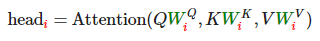
ViT 과제
- Vision + Transformer
- 구성
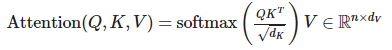
- Image Embedding
-
기존 NLP에서는 나열된 문장이 입력 / 이미지를 입력으로 사용하기 위해서, 여러개의 Patch로 나눕니다.
-
마지막 Classification을 위해, 나눠진 Patch의 맨 앞에 Special Token 추가
-
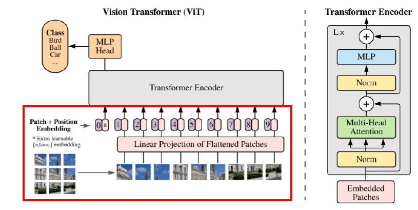
- Transformer Encoder
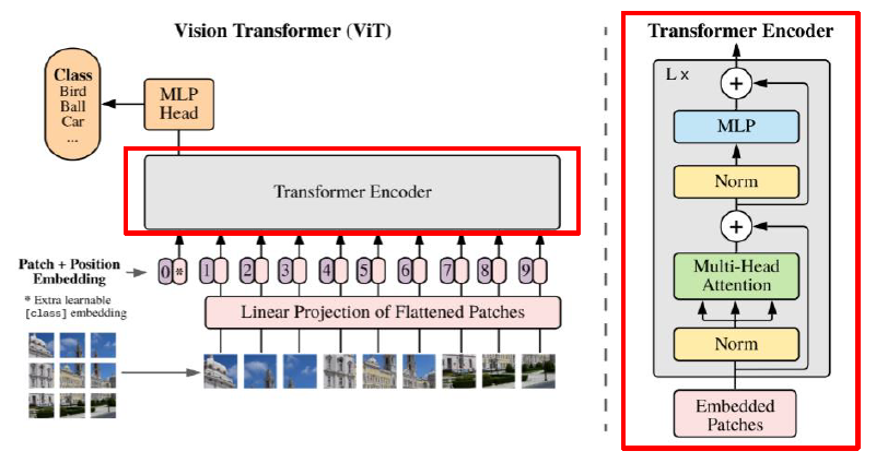
- Classification
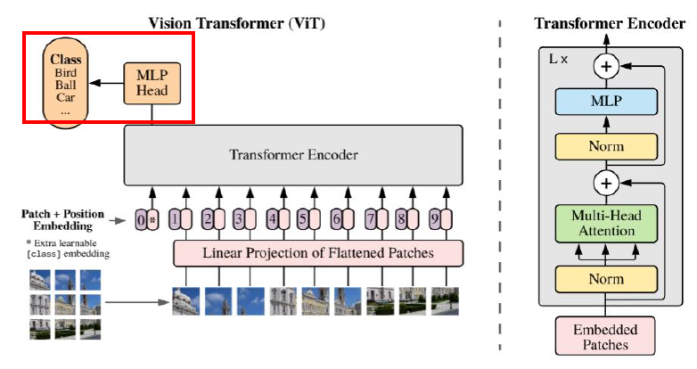
- Image Embedding
-
코드
- Image(Patch) Imbedding

c = repeat(cls_token, ‘() n d → b n d’, b=batch)x = torch.cat((c, x), dim=1)x = x + positions
- Transformer
- Encoder (MHA)
# query, key , value
Q = self.query(x)
K = self.key(x)
V = self.value(x)

Q = rearrange(Q, 'b q (h d) -> b h q d', h=self.num_heads)
K = rearrange(K, 'b k (h d) -> b h d k', h=self.num_heads)
V = rearrange(V, 'b v (h d) -> b h v d', h=self.num_heads)

# scaled dot-product
weight = torch.matmul(Q, K)
weight = weight * self.scaling

attention = torch.softmax(weight, dim=-1)
attention = self.att_drop(attention)

context = torch.matmul(attention, V)
context = rearrange(context, 'b h q d -> b q (h d)')

x = self.linear(context)
- Encoder (MHA)
- Classification
x = linear_1(x)x = nn.functional.gelu(x)x = dropout(x)x = linear_2(x)
- Image(Patch) Imbedding
-
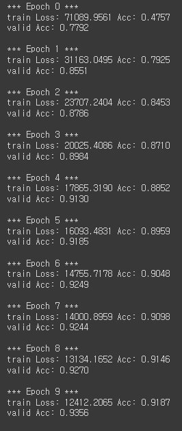
Train
- 성능: 대표적인 Image Classification Task인 ImageNet에서 좋은 성능 기록
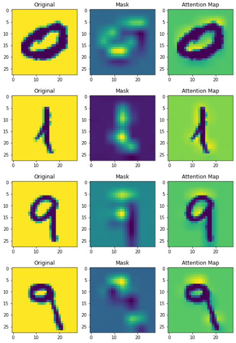
- 추가 Tip
- 시각화 도구를 이용하여 feature map을 뽑아볼 수 있다.
- 9의 경우를 보면 9의 feature가 어느 부분인지 확인 가능하다!
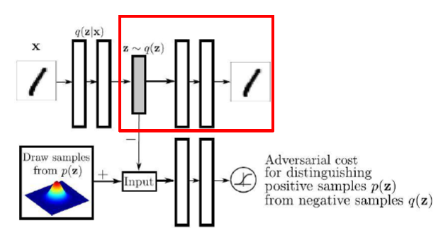
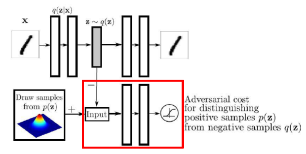
AAE 과제
- Adversarial Autoencoder
- 구성
- Encoder (Generator in GAN)
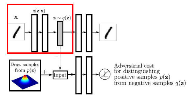
- Decoder
- Discriminator
- Encoder (Generator in GAN)
- 코드
- Encoder
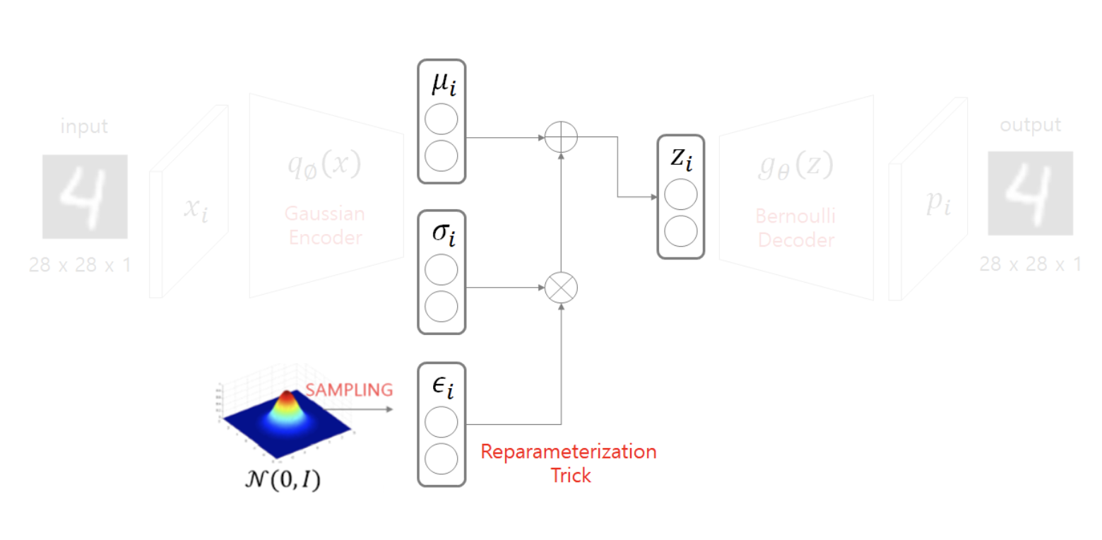
# model self.model = nn.Sequential( nn.Linear(1024, 512), nn.Dropout(p=0.2), nn.ReLU(), nn.Linear(512, 512), nn.Dropout(p=0.2), nn.ReLU() ) self.mu = nn.Linear(512, latent_dim) self.logvar = nn.Linear(512, latent_dim) # forward img_flat = img.view(img.shape[0], -1) x = self.model(img_flat) mu = self.mu(x) logvar = self.logvar(x) z = reparameterization(mu, logvar)- Reparametrization
-
Decoder에 들어가기 전, Encoder 아웃풋인 μ(mu)와 σ(sigma)가 나오게 된다. p(z)에서 샘플링을 할때, 데이터의 확률 분포와 같은 분포에서 샘플을 뽑아야하는데, backpropagation을 하기 위해선, reparametrization의 과정을 거친다.
-
즉, 정규분포에서 z를 샘플링 하는 것
-
- Reparametrization
- Decoder
# model self.model = nn.Sequential( nn.Linear(latent_dim, 512), nn.Dropout(p=0.2), nn.ReLU(), nn.Linear(512, 512), nn.BatchNorm1d(512), nn.Dropout(p=0.2), nn.ReLU(), nn.Linear(512, 1024), nn.Tanh(), ) # forward q = self.model(z) q = q.view(q.shape[0], *img_shape) - Discriminator
self.model = nn.Sequential(
    nn.Linear(latent_dim, 512),
    nn.Dropout(p=0.2),
    nn.ReLU(),
    nn.Linear(512, 256),
    nn.Dropout(p=0.2),
    nn.ReLU(),
    nn.Linear(256, 1),
    nn.Sigmoid(),
)

# forward
x = self.model(z)
- Encoder
- Train
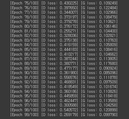
- 결과
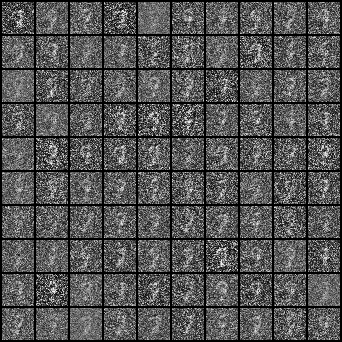
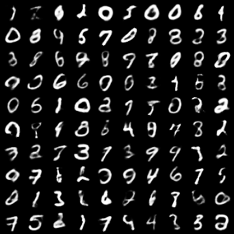 노이즈로부터 차근히 학습되어 생성된 결과를 확인할 수 있다.

함께 자라기