이 글은 Linear Algebra and Its Applications 책을 정리한 글입니다.

• 어떠한 inconsistent system of equation이 solution이 없을때 approximate solution을 구할 필요가있다. 이번 챕터에서는 orthogonality라는 성질을 통해 nearest point를 찾고 approximate solution을 찾을것 이다.

6.1 Inner product, length, and orthogonality

---

The Inner Product

• 위와같은 $\mathbb{R}^n$ 의 vector $\bold{u, v}$가 있을때 우리는 이를 $n \times 1$ matrix로 간주할 수 있으며, tranpose인 $\bold{u}^T$를 $1 \times n$ matrix이다. 또한 이들의 matrix product인 $\bold{u}^T\bold{v}$ 는 a single real number로 쓸 수 있는데 이를 Inner product라고 하며 $\bold{u}^T\sdot\bold{v}$ 라고 쓸 수 있으며 이를 dot product라고 한다.

Theorem1
Let $\bold{u, v, w}$ be vector in $\mathbb{R}^n$, and let c be scalar then,

• $\bold{u} \sdot \bold{v}$ = $\bold{v} \sdot \bold{u}$
• $(\bold{u} + \bold{v})\sdot \bold{w} = \bold{u}\sdot \bold{w} + \bold{v}\sdot \bold{w}$
• $(c\bold{u})\sdot\bold{v} = c(\bold{u}+\bold{v})$
• $\bold{u}\sdot \bold{u} \ge 0$ and $\bold{u}\sdot \bold{u} = 0$ if and only if $\bold{u} = 0$

The Length of a Vector

Definition

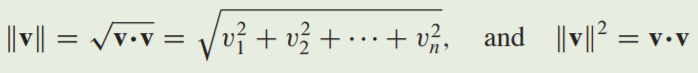
• The length (or norm) of $\bold{v}$ in $\mathbb{R}^n$ is nonnegative scalar $\rVert\bold{v}\lVert$ defined by
  
• $\rVert c\bold{v}\lVert = \rVert c\lVert\rVert \bold{v}\lVert$
• unit vector $\to$ $\rVert\bold{u}\lVert$ = 1
• normalizationing $\to$ $\bold{u} = \frac{1}{\rVert\bold{v}\lVert}\bold{v}$

Distance in $\mathbb{R}^n$

Definition

• For $\bold{u}$ and $\bold{v}$ in $\mathbb{R}^n$, the distance between $\bold{u}$ and $\bold{v}$, written as dist($\bold{u}$,$\bold{v}$), is the length of the vector $\bold{u}-\bold{v}$. That is dist($\bold{u}$,$\bold{v}$) = $\lVert\bold{u}-\bold{v}\rVert$

Example

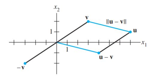
• 두 vector $\bold{u} = (7,1)$, $\bold{v} = (3,2)$ 사이의 distance를 구하라.

• 아래 그림에서 나타나다시피 $\bold{u}$와 $\bold{v}$의 distance는 $\bold{u-v}$ 와 0 사이의 distance와 같다.

Example4

Orthogonal Vectors

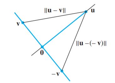
• 위 그림에서 distance from $\bold{u}$ to $\bold{v}$ 이 distance from $\bold{u}$ to $-\bold{v}$랑 같다묜 이는 geometrically perpendicular하며 이 둘은 squares of distance가 같다.

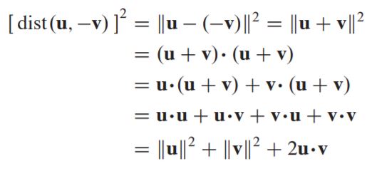
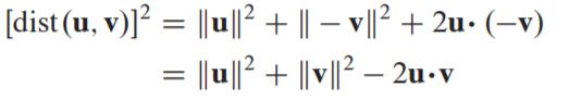
• 두 dist가 같을 조건은 2$\bold{u}\sdot\bold{v}$ = -2$\bold{u}\sdot\bold{v}$ 이므로 $\bold{u}\sdot\bold{v} = 0$
  이 되어야한다.

Definition
-Two vectors $\bold{u}$ and $\bold{v}$ in $\mathbb{R}^n$ are orthogonal if $\bold{u}\sdot\bold{v} = 0$

• 추가로 zero vector는 $\mathbb{R}^n$의 모든 vector에 대하여 orthogonal하다 ($\bold{0}^T\sdot\bold{v} = 0$)

Theorem
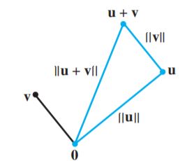
Pythagoream Theorem

• Two vector $\bold{u, v}$ are orthogonal if and only if $\lVert\bold{u+v}\rVert^2 = \lVert\bold{u}\rVert^2 + \lVert\bold{v}\rVert^2$

Orthogonal Complement

• vector $\bold{z}$가 $\mathbb{R}^n$의 subspace W에 모든 vector에 orthogonal하다면, $\bold{z}$는 W에 orthogonal하다고 말한다. 또한 W에 orthogonal인 set of all vector $\bold{z}$를 orthogonal complemnet of W 라고 하며 $W^\bot$으로 표기한다.

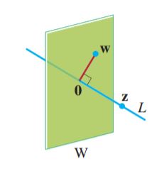
• 위 그림처럼 W가 $R^3$의 원점을 지나는 subspace인 평면이고 L이 W에 perendicular(직각)이며 원점을 지나는 직선이다. vector $\bold{z}$가 W of $\mathbb{R}^3$의 모든 벡터에 orthogonal한다면 $\bold{z}$는 orthogonal to W라고 부른다 ($\bold{z}\sdot$W = 0).
  - ortogonal이 vector관의 관계 뿐 아니라 벡터와 subspace사이에서도 사용됨.

Example

• vector $\bold{y}$ 가 vectors $\bold{u}$ and $\bold{v}$에 orthogonal하다고 가정했을때. $\bold{y}$ 가 vector $\bold{u + v}$에 orthogonal함을 보여라.

Example6~8

Theorem3

• Let A be an $n \times n$ matrix. The orthogonal complement of the row space of A is the null space of A, and the orthogonal complement of the column space of A is the null space of $A^\top$ :

6.2 Orthogonal Sets

---

• A Set of vectors ${\bold{u}_1, \ \dots, \ \bold{u}_p}$ in $\mathbb{R}^n$ is said to be an orthogonal set if each pair of distinct vectors from the set is orthogonal, if $\bold{u}_i \sdot \bold{u}_j = 0$ whenever $i \ne j$
  - 해당 set안의 임이의 두 vector가 orthogonal하아면 그 set은 orthogonal set이다는 소리.

Example

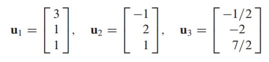
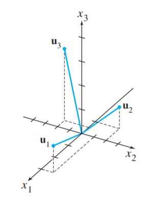
• 위 세 vector set이 orthogonal set인지 보여라.

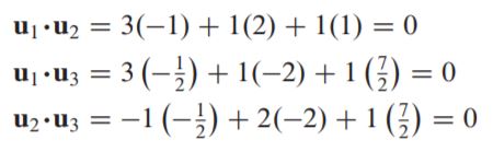
• 각각의 vector들이 orthogonal함을 보였으니 이는 orthogonal set이며 아래 그림과 같다.

Theorem

• If S = {$\bold{u}_1, \ \dots, \ \bold{u}_p$} is an orthogonal set of nonzero vectors in $\mathbb{R}^n$, then S is linearly independent and hence is a basis for the subspace spanned by S.

• 위 식인 linear combination을 만족하는 $c_1$ ~ $c_p$가 0인 경우 linearly independent set임을 보일 수 있다.

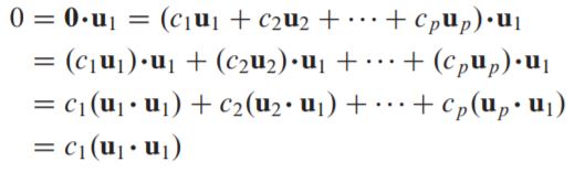
• 위처럼 양변에 $\bold{u}_1$을 dot product 시키면 $c_1(\bold{u}_1 \sdot \bold{u}_1) = 0$ 이 되고, 이때 $\bold{u}_1 \sdot \bold{u}_1$는 당연하게도 무조건 0이상이기에 $c_1 = 0$이 된다.

Definition
Orthogonal Basis

• An orthogonal basis for a subspace W of $\mathbb{R}^n$ is a basis for W that is also an orthogonal set.

• $\mathbb{R}^n$의 subspace의 basis이면서 orthogoanl set이면 orthogonal basis라는 소리.

Theorem

• Let {$\bold{u}_1, \ \dots, \ \bold{u}_p$} be an orthogonal basis for a subspace W of $\mathbb{R}^n$. For each $\bold{y}$ in W , the weights in the linear combination $\bold{y} = c_1\bold{u}_1 + \dots + c_p\bold{u}_p$ are given by $c_j = \frac{\bold{y} \sdot \bold{u}_j}{\bold{u}_j \sdot \bold{u}_j}$.

• 이 전까지 weights를 찾으려면 augmented matrix를 row operation하여 solution을 찾았는데 orthogonal basis이면 위처럼 명시적으로 주어진다.

• 위 식에서 orthogonal set이기에 $\bold{u}_1$ 끼리의 dot product빼고는 전부 0이 된다.

Example

• set S = {$\bold{u}_1, \ \bold{u}_2, \ \bold{u}_3$}이 위와 같고, orthogonal basis for $\mathbb{R}^3$일때 vector $\bold{y}$ = (6,1,-8)를 orthogoanl basis로 표현해보자.

• 간단하게 위 이론에서처럼 계산해보면 위와같다.

Orthogonal Projection

• nonzero vector $\bold{u}$ in $\mathbb{R}^n$이 주어졌고 vector $\bold{y}$ in $\mathbb{R}^n$ 을 두 벡터로 decomposing해보면 아래처럼 나타낼 수 있고,

• some scalar $\alpha$에 $\bold{\hat{y}} = \alpha\bold{u}$ 이고 $\bold{z}$ 가 $\bold{u}$에 orthogonal 할때 $\bold{z} = \bold{y} - \alpha\bold{u}$라면 위 식을 만족한다.

• 이때 $\bold{y - \hat{y}}$ 이 $\bold{u}$에 orthogonal하다면,
  $0 = (\bold{y} - \alpha\bold{u})\sdot\bold{u} = \bold{y}\sdot\bold{u} - (\alpha\bold{u})\sdot\bold{u} = \bold{y}\sdot\bold{u} - \alpha(\bold{u}\sdot\bold{u})$ 가 되며 이때, $\alpha = \frac{\bold{y}\sdot\bold{u}}{\bold{u}\sdot\bold{u}}$ 이고 $\bold{\hat{y}} = \frac{\bold{y}\sdot\bold{u}}{\bold{u}\sdot\bold{u}}\bold{u}$ 이 된다.

• 이때 vector $\bold{\hat{y}}$ 는 orthogonal projection of y onto u 로 부르며, vector $\bold{z}$를 component of y orthogonal to u 라고 하며 vector를 subspace L ( span{$\bold{u}$} )로 확장하면 다음과같이 나타낼 수 있다.

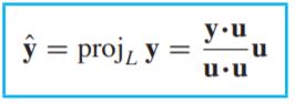
* 위 내용은 어떤 vector가 있을 때 어떤 다른 vector 혹은 그 vector의 span에다 orthogonal projection이 어떤식으로 정의되는지를 보여준 것이다.

Example

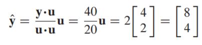
• 아래 두 vector가 주어졌을때 orthogonal projection of $\bold{y}$ onto $\bold{u}$를 찾고 $\bold{y}$ 를 두 orthogonal vector의 합으로 나타내라 (하나는 in Span{$\bold{y}$}, 다른 하나는 orthogonal to $\bold{u}$)

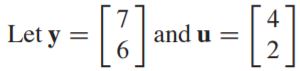
• orthogonal projection of $\bold{y}$ onto $\bold{u}$ 인 $\bold{\hat{y}}$ 를 구하기위해 계산하면 다음과같고,

• component of $\bold{y}$ orthogonal to $\bold{u}$ (orthogonal to $\bold{u}$) 를 구하면 다음과 같다.

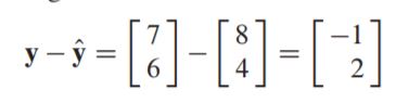
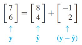
• $\bold{y}$ 를 두 벡터로 나타내면 다음과같다.

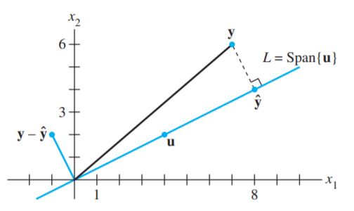
• 이를 그림으로 나타내면 다음과 같다.

Orthonomal sets

• A Set {$\bold{u_1}, \dots, \bold{u_p}$} is an orthonormal set if it is an orthogonal set of unit vectors.
  - 다시 언급하면 unit vector는 vector의 norm(length)이 1인 vector

Theorem

• An $m \times n$ matrix $U$ has orthonormal columns if and only if $U^\top U = I$

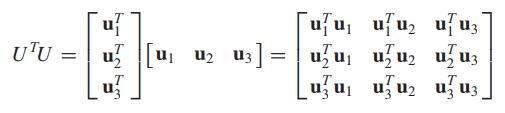
• $U^\top U$ 를 위와같이 전개하여 보면 diagonal term들이 전부 1이고 나머지 entry가 0이면 $U$는 orthonomal columns를 갖는단 소리.

Theorme

• Let $U$ be an $m \times n$ matrix with orthonormal columns, and let $\bold{x}$ and $\bold{y}$ be in $\mathbb{R}^n$. Then
  
  a. $\lVert U\bold{x} \rVert = \lVert \bold{x} \rVert$
  b. $(U\bold{x})\sdot(U\bold{y}) = \bold{x \sdot y}$
  c. $(U\bold{x})\sdot(U\bold{y}) = 0$ if and only if $\bold{x \sdot y} = 0$

6.3 Orthogonal Projection

---

• vector $\bold{y}$와 subspace W in $\mathbb{R}^n$ 이며 $\bold{y} - \hat\bold{y}$ 이 W에 orthogonal할때 unique vector $\hat\bold{y}$ 가 있다. 이는 후에 다룰 least-squares solution에서 중요하게 다뤄진다.

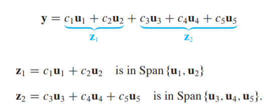
• vector $\bold{y}$ 는 vectors $\bold{u}_1, \ \dots, \ \bold{u}_n$ 의 linear combination으로 나타내었을 때 $\bold{y}$ 는 $\bold{y} = \bold{z}_1 + \bold{z}_2$ 처럼 두개의 그룹으로 나타낼 수 있는데 이때 $\bold{z}_1$ 은 linear combination의 일부이며 $\bold{z}_2$는 linear combination의 나머지이다. 이는 {$\bold{u}_1, \ \dots, \ \bold{u}_n$} 가 orthogoanl basis( $W^\perp$ ) 일때 유용하게 사용된다.

Example

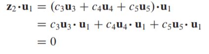
• {$\bold{u}_1, \ \dots, \ \bold{u}_5$} 가 $\mathbb{R}^5$ 의 orthogonal basis이며 $\bold{y} = c_1\bold{u}_1 + \dots + c_5\bold{u}_5$ 이고 subspace W = Span{$\bold{u}_1, \bold{u}_2$} 이라고 하였을때 $\bold{y}$ 는 vector $\bold{z}_1$ in W와 vector $\bold{z}_2$ in $W^\perp$ 로 아래와같이 나타낼 수 있다.

• $\bold{z}_2$ in $W^\perp$ 을 보이기 위해선 $\bold{z}_2$ 가 basis {$\bold{u}_1, \bold{u}_2$} for W의 vector에 대해 orthogonal함을 보이면 된다.

Theorme

• Let W be a subspace of $\mathbb{R}^n$. Then each $\bold{y}$ in $\mathbb{R}^n$ can be written uniquely in the form $\bold{y} = \hat\bold{y} + \bold{z}$, where $\hat\bold{y}$ is in W and $\bold{z}$ is in $W^\perp$. In fact, if {$\bold{u}_1, \ \dots, \ \bold{u}_p$} is any orthogonal basis of W, then $\hat\bold{y} = \frac{\bold{y} \sdot \bold{u}_1}{\bold{u}_1 \sdot \bold{u}_1}\bold{u}_1 + \dots + \frac{\bold{y} \sdot \bold{u}_p}{\bold{u}_p \sdot \bold{u}_p}\bold{u}_p$ and $\bold{z} = \bold{y} - \hat\bold{y}$.

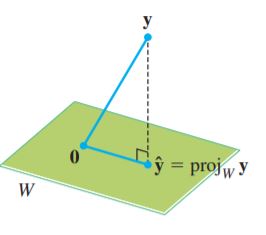
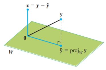
• The vector $\hat\bold{y}$ 는 orthogonal projection of y onto W 라고 하며 $proj_w\bold{y}$로 나타내며 아래의 그림과같다.
  - 이는 이전에 보았던 orthogonal projection of y onto L 을 subspace로 확장한것.
  

Example

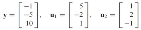
• 아래와 같이 vector가 주어졌고 {$\bold{u_1, u_2}$} 가 orthogoanl basis for W = Span{$\bold{u_1, u_2}$} 일때 $\bold{y}$ 를 W의 vector와 W에 orthogonal한 vector의 합으로 나타내라.

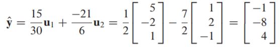
• theorme에 따라 $\bold{\hat{y}}$ 을 구하고 $\bold{y - \hat{y}}$ 을 구하면 다음과 같고

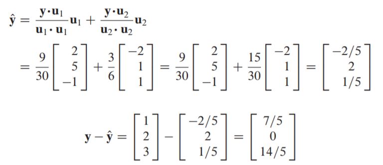
• y를 두 vector의 합으로 decompose시키면 다음과 같다.

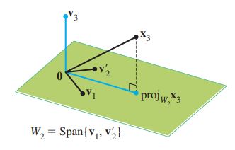
A Geometric Interpretation of the Orthogonal Projection

• 이번엔 이전까지 보았던 $\mathbb{R}^2$ space를 확장해 $\mathbb{R}^3$ space상에서 시각적으로 살펴본다.

• $\mathbb{R}^3$ space의 임의의 vector $\bold{y}$를 Span{$\bold{u_1, u_2}$} 평면에 orthogonal projection 시켜보자.

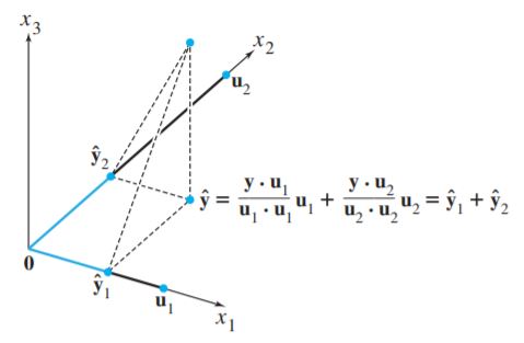
• 위 그림처럼 $\hat\bold{y}$는 $\frac{\bold{y} \sdot \bold{u}_1}{\bold{u}_1 \sdot \bold{u}_1}\bold{u}_1 + \frac{\bold{y} \sdot \bold{u}_2}{\bold{u}_2 \sdot \bold{u}_2}\bold{u}_2$로 정의에서처럼 명시할 수 있고 이때 각각의 component는 $\hat\bold{y}_1$, $\hat\bold{y}_2$ 로 나누어지며 이 $\hat\bold{y}_1$, $\hat\bold{y}_2$는 결국 orthogonal basis의 각 벡터 ($\bold{u_1, u_2}$) 가 span 하는 Line에 orthogonal projection 시킨 것 이다.

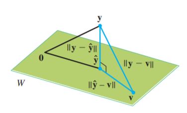
Theorme - The best approximation theorem

• Let $W$ be a subspace of $\mathbb{R}^n$, $\bold{y}$ any vector in $\mathbb{R}^n$, and $\hat\bold{y}$ be the orthogonal projection of $\bold{y}$ onto $W$. Then $\hat\bold{y}$ is the colset point $W$ to $\bold{y}$, in the sense that $\lVert \bold{y} - \hat\bold{y} \rVert < \lVert \bold{y} - \bold{v} \rVert$ for all $\bold{v}$ in $W$ distinct from $\hat\bold{y}$.

• length 측면으로 보았을때 $\bold{y}$ 와 $\hat\bold{y}$간의 차이가 $W$에 어떤 vector $\bold{v}$와의 차보다 작다는 뜻으로 아래 그림을 보고 이해할 수 있다.

Example

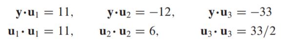
• 아래와 같이 vector $\bold{u_1, u_2, y}$ 가 주어지고 $W$가 Span{$\bold{u_1, u_2}$} 이고 $\bold{y}$가 nearest point to $W$라고 하였을 때 distance from $\bold{y}$ to $W$ 를 구해라.

• $\lVert \bold{y} - \hat\bold{y} \rVert$ 를 구하기 위해 $\hat\bold{y}$를 구하면 다음과 같고

• distance를 구하면 다음과같다.

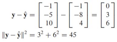
• $\therefore$ distance from $\bold{y}$ to $W$ = $3\sqrt5$

Theorme

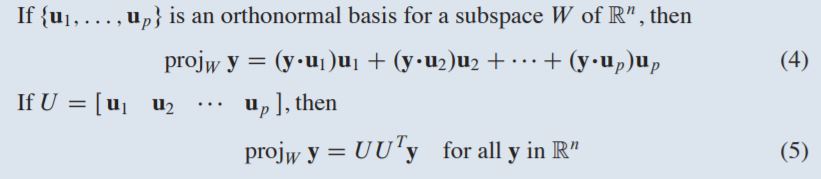
• 일단 $\bold{u_1}$ ~ $\bold{u_p}$ 가 orthonomal basis이기에 $proj_W{\bold{y}}$ 에서 각 vector의 coefficient의 분모가 unit vector끼리의 dot product이니 1이되어 위 (4)식으로 나타낼 수 있다.

• 또한 $proj_W{\bold{y}}$ = $UU^\top\bold{y}$ 로 쓸 수있는데 이는 (4)번 식을 dot product 정의에 의해 $(\bold{u^\top_1 y})\bold{u}_1$ 로 나타낼 수 있고 이를 matrix로 정리하여 y를 바깥으로 빼내면 $UU^\top\bold{y}$로 나타낼 수 있다.

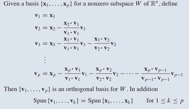
6.4 The Gram-Schmidt Process

---

• 이전까진 subspace를 이루는 orthogonal basis가 주어졌을 때 를 가정하였지만 이번 챕터는 gram-schmidt 라는 방법을 통해 orthogonal basis를 구하는 방법을 볼 것이다.

• vector {$\bold{v_1, v_2}$}를 subspace $W$ = Span{$\bold{v_1, v_2}$}의 basis라고 가정하자
  - Span{$\bold{v_1, v_2}$}의 basis가 orthogonal하다는 말이 없으니 orthogonal set이 아니라 그냥 linearly independent set이다.

• 이때 subspace $W$를 이루는 orthogonal basis를 찾아보자.

• $\bold{v}_1$을 $\bold{u}_1$이라고 하고 $\bold{v}_2$를 $\bold{u}_1$에 projection 시켜 $\hat\bold{v}_2$ ($proj_{\bold{u_1}}\bold{v_2}$)를 구한 후 $\bold{u}_2$ 를 $\bold{v}_2 - \hat\bold{v}_2$ 로 나타낼 수 있다.

• 이때 $\bold{u}_2 = \bold{v}_2 - \hat\bold{v}_2 = \bold{v}_2 - \frac{\bold{v}_2 \sdot \bold{v}_1}{\bold{v}_1 \sdot \bold{v}_1}\bold{v}_1$ 의 linear combination 형태로 나타날수 있으므로 $\bold{u}_2$는 subspace $W$에 있다는 것을 알수 있다.

• $\bold{u}_1$, $\bold{u}_2$가 $W$에 있음을 보였고 orthogonal하게 만들었으니 $\bold{u}_1$은 당연히 nonzero이고 $\bold{u}_2$가 nonzero임을 보여 linearly independent 함을 보여야한다 ($\bold{u}_1$과 $\bold{u}_2$가 orthogonal set이기에 nonzero이면 당연히 independent하다) .

• 만일 $\bold{u}_2$가 nonzero가 아니라면 $\bold{v}_2$ 와 $\hat\bold{v}_2$이 같다는 것인데 이는 $\bold{v}_2$가 Span{$\bold{v}_1$} 에 있다는 뜻이므로 둘은 dependent set이되고 이는 처음 정의에 의해 $\bold{v}_1$과 $\bold{v}_2$ 가 subspace의 basis이니 성립이되지 않아 둘은 linearly independent하다.

  $\therefore$ W = Span{$\bold{u_1, u_2}$} = Span{$\bold{v_1, v_2}$}

• $\mathbb{R}^3$ space의 orthogonal basis를 찾는것도 똑같다.

• 벡터 이름이 바뀌어 햇갈리지만 이번엔 basis를 이루는 또다른 주어진 벡터 $\bold{x}_3$를 $\mathbb{R}^2$ space 에서 구한 평면 $W$ (위 그림에선 $W_2$) 에 projection시켜 $\bold{v_3}$를 찾으면 된다.

• 그 다음엔 $\bold{v_3} = \bold{x_3} - \hat\bold{x}_3$을 구하면 되는데 $\hat\bold{x}_3$는 이 전 챕터에서 한 것 처럼 $\bold{v_1}$과 $\bold{v_2}$에 projection시켜주면 된다.

Theorem - The Gram-Schmidt Process

• 위 내용처럼 $\mathbb{R}^n$ space의 subspace $W$의 basis로 하나씩 projection시켜주며 $\bold{v}_p$ 까지 구하여 $W$의 orthogonal basis를 찾을 수 있다.

• 또한 $\bold{v}_1$ ~ $\bold{v}_p$까지를 구할때 $\bold{v}_k$는 $\bold{v}_1$ ~ $\bold{v}_{k-1}$과 $\bold{x}_k$의 linear combination으로 나타낼수 있었고 이를통해 Span{$\bold{v_1, \dots, v_k}$} = Span{$\bold{x_1, \dots, x_k}$} 임을 알 수 있다.

Orthonormal basis

• Orthonomal basis는 말 그대로 orthogonal basis에서 각각의 vector들의 norm을 1로 만들어 normalize 시킨 것 이다.

QR Factorization of Matrices

Theorme - The QR Factorization

• If A is an $m \times n$ matrix with linearly independent columns, then A can be factored as A = QR, where Q is an $m \times n$ matrix whose columns form an orthonormal basis for Col A and R is an $n \times n$ upper triangular invertible matrix with positive entries on its diagonal.

• $m \times n$ matrix A가 linearly independent coulmns를 갖고있다 했으니 이는 A = [$\bold{x}_1 \ \bold{x}_2 \ \dots \ \bold{x}_n$]으로 나타낼 수 있고 이때의 Col A 의 basis는 {$\bold{x}_1, \dots, \bold{x}_n$}가 되며 이를 Gram-Schmidt를 통해 구한 Col A의 orthonormal basis를 {$\bold{u}_1, \ \dots, \ \bold{u}_n$} 이라고 하자.

• 이때 Col A의 orthonormal basis를 columns 으로 둔 matrix 를 Q라 하고 다음과같이 나타낼수 있다 Q = [$\bold{u}_1 \ \bold{u}_2 \ \dots \ \bold{u}_n$].

• 이전에 배웠던 것처럼 $\bold{x}_k$ = $\bold{u}_1, \dots, \bold{u}_k$으로 나타낸 linear combination 임을 알 수 있고 $\bold{x}$가 n까지 나타날수 있으니 아래 식처럼 나타낼 수 있다.

• 이때 vector $\bold{r}_k$를 아래와같이 나타낼 수 있으며,

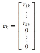
• 이는 $\bold{x}_k$ = Q$\bold{r}_k$ 식으로 나타낼 수 있고 이를통해 아래와 같이 유도된다.

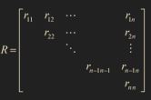
• 이때 A의 column들이 linealy independent하니 R은 invertible matrix가 되며 이는 n개의 pivot을 갖는단 소리고 이는 R의 diagonal term들이 nonzero가 되어 아래 그림처럼 upper triangular matrix가 된다.

• 또한 $(-\bold{r}_{kk})(-\bold{u}_k)$ 처럼 unit vector에 방향을 바꿔주어 R의 diagonal term을 nonnegative하게 만들 수 있다.

• 또한 이전에 보았던 $U^\top U = I$ 이론을 통해 $Q^\top A = Q^\top(QR) = R$ 과 같이 A에 $Q^\top$를 multiplication해주어 R을 찾을 수 있다.