[논문 번역] Swin Transformer: Hierarchical Vision Transformer using Shifted Windows

Swin Transformer: Hierarchical Vision Transformer using Shifted Windows
Abstract
This paper presents a new vision Transformer, called Swin Transformer, that capably serves as a general-purpose backbone for computer vision.
이 논문은 Swin Transformer라는 새로운 비전 트랜스포머를 소개하며, 이는 범용 컴퓨터 비전 백본으로 효과적으로 활용될 수 있다.
Challenges in adapting Transformer from language to vision arise from differences between the two domains, such as large variations in the scale of visual entities and the high resolution of pixels in images compared to words in text.
텍스트 기반의 트랜스포머를 비전 영역에 적용할 때는, 시각적 객체의 크기 변화가 매우 크고 이미지의 픽셀 해상도가 텍스트 단어보다 훨씬 높다는 등 두 도메인 간 차이로 인해 어려움이 발생한다.
To address these differences, we propose a hierarchical Transformer whose representation is computed with Shifted windows.
이러한 차이를 해결하기 위해, 우리는 Shifted window 구조로 표현을 계산하는 계층형 트랜스포머를 제안한다.
The shifted windowing scheme brings greater efficiency by limiting self-attention computation to non-overlapping local windows while also allowing for cross-window connection.
Shifted window 방식은 self-attention을 겹치지 않는 로컬 윈도우로 제한하여 효율성을 높이면서도, 윈도우 간 연결을 가능하게 한다.
This hierarchical architecture has the flexibility to model at various scales and has linear computational complexity with respect to image size.
이 계층적 아키텍처는 다양한 스케일을 모델링할 수 있는 유연성을 제공하며, 이미지 크기에 대해 선형적인 계산 복잡도를 가진다.
These qualities of Swin Transformer make it compatible with a broad range of vision tasks, including image classification (87.3 top-1 accuracy on ImageNet-1K) and dense prediction tasks such as object detection (58.7 box AP and 51.1 mask AP on COCO test-dev) and semantic segmentation (53.5 mIoU on ADE20K val).
이러한 특성 덕분에 Swin Transformer는 이미지 분류(Imagenet-1K 기준 Top-1 정확도 87.3), 객체 탐지(COCO test-dev 기준 box AP 58.7, mask AP 51.1), 시맨틱 세그멘테이션(ADE20K val 기준 mIoU 53.5) 등 다양한 비전 작업에 적합하다.
Its performance surpasses the previous state-of-the-art by a large margin of +2.7 box AP and +2.6 mask AP on COCO, and +3.2 mIoU on ADE20K, demonstrating the potential of Transformer-based models as vision backbones.
Swin Transformer는 COCO에서 기존 SOTA 대비 box AP +2.7, mask AP +2.6, ADE20K에서 mIoU +3.2를 크게 향상시키며, 트랜스포머 기반 모델이 비전 백본으로서 가지는 잠재력을 입증한다.
The hierarchical design and the shifted window approach also prove beneficial for all-MLP architectures.
이 계층적 설계와 Shifted window 접근법은 순수 MLP 기반 아키텍처에도 유용하다는 것이 확인되었다.
The code and models are publicly available at https://github.com/microsoft/Swin-Transformer.
코드와 모델은 https://github.com/microsoft/Swin-Transformer 에 공개되어 있다.
1. Introduction
Modeling in computer vision has long been dominated by convolutional neural networks (CNNs).
컴퓨터 비전 분야에서의 모델링은 오랫동안 합성곱 신경망(CNN)이 주도해왔다.
Beginning with AlexNet [39] and its revolutionary performance on the ImageNet image classification challenge, CNN architectures have evolved to become increasingly powerful through greater scale [30, 76], more extensive connections [34], and more sophisticated forms of convolution [70, 18, 84].
ImageNet 이미지 분류 대회에서 혁신적인 성능을 보인 AlexNet [39] 이후, CNN 구조는 규모 확장 [30, 76], 더 복잡한 연결 구조 [34], 더욱 정교한 합성곱 방식 [70, 18, 84]을 통해 점점 강력하게 발전해왔다.
With CNNs serving as backbone networks for a variety of vision tasks, these architectural advances have led to performance improvements that have broadly lifted the entire field.
CNN이 다양한 비전 작업의 백본 네트워크로 활용되면서, 이러한 구조적 발전은 전반적인 성능 향상을 이끌어 전체 분야 발전에 크게 기여했다.
On the other hand, the evolution of network architectures in natural language processing (NLP) has taken a different path, where the prevalent architecture today is instead the Transformer [64].
반면, 자연어 처리(NLP)의 네트워크 아키텍처 발전은 다른 방향을 따랐으며, 현재 NLP에서는 Transformer [64]가 지배적인 구조로 자리 잡았다.
Designed for sequence modeling and transduction tasks, the Transformer is notable for its use of attention to model long-range dependencies in the data.
Transformer는 시퀀스 모델링과 변환 작업을 위해 설계되었으며, 데이터의 장기 의존성을 모델링하기 위해 어텐션 메커니즘을 사용하는 점이 특징이다.
Its tremendous success in the language domain has led researchers to investigate its adaptation to computer vision,
Transformer가 언어 분야에서 거둔 큰 성공은 연구자들로 하여금 이를 컴퓨터 비전에 적용하려는 시도를 촉진했다.
where it has recently demonstrated promising results on certain tasks, specifically image classification [20] and joint vision-language modeling [47].
그리고 최근에는 특정 작업, 특히 이미지 분류 [20]와 비전-언어 결합 모델링 [47]에서 유망한 성과를 보이고 있다.
In this paper, we seek to expand the applicability of Transformer such that it can serve as a general-purpose backbone for computer vision, as it does for NLP and as CNNs do in vision.
본 논문에서는 Transformer가 NLP에서 그러하듯, 그리고 CNN이 비전에서 그러하듯, 컴퓨터 비전에서도 범용 백본으로 활용될 수 있도록 적용 범위를 확장하고자 한다.
We observe that significant challenges in transferring its high performance in the language domain to the visual domain can be explained by differences between the two modalities.
언어 분야에서의 높은 성능을 시각 분야로 그대로 이전하는 데에는 두 모달리티 간의 차이에서 비롯된 여러 문제가 존재함을 확인했다.
One of these differences involves scale.
그 차이 중 하나는 ‘스케일’ 문제이다.
Unlike the word tokens that serve as the basic elements of processing in language Transformers, visual elements can vary substantially in scale, a problem that receives attention in tasks such as object detection [42, 53, 54].
언어 Transformer의 기본 요소인 단어 토큰과 달리, 시각적 요소는 스케일이 매우 다양하며 이는 객체 탐지 [42, 53, 54]와 같은 작업에서 중요한 문제로 다뤄진다.
In existing Transformer-based models [64, 20], tokens are all of a fixed scale, a property unsuitable for these vision applications.
하지만 기존 Transformer 기반 모델 [64, 20]에서는 모든 토큰이 동일한 스케일을 가지며, 이는 이러한 비전 작업에 적합하지 않다.
Another difference is the much higher resolution of pixels in images compared to words in passages of text.
또 다른 차이점은 이미지의 픽셀 해상도가 텍스트 단어보다 훨씬 높다는 점이다.
There exist many vision tasks such as semantic segmentation that require dense prediction at the pixel level, and this would be intractable for Transformer on high-resolution images, as the computational complexity of its self-attention is quadratic to image size.
시맨틱 세그멘테이션처럼 픽셀 단위의 조밀한 예측이 필요한 비전 작업이 많으며, Transformer의 self-attention 복잡도가 이미지 크기에 대해 이차적으로 증가하기 때문에 고해상도 이미지에서는 계산이 사실상 불가능하다.
To overcome these issues, we propose a general-purpose Transformer backbone, called Swin Transformer, which constructs hierarchical feature maps and has linear computational complexity to image size.
이 문제들을 해결하기 위해, 우리는 계층적(feature hierarchical) 특성 맵을 구성하고 이미지 크기에 대해 선형 복잡도를 가지는 범용 Transformer 백본인 Swin Transformer를 제안한다.
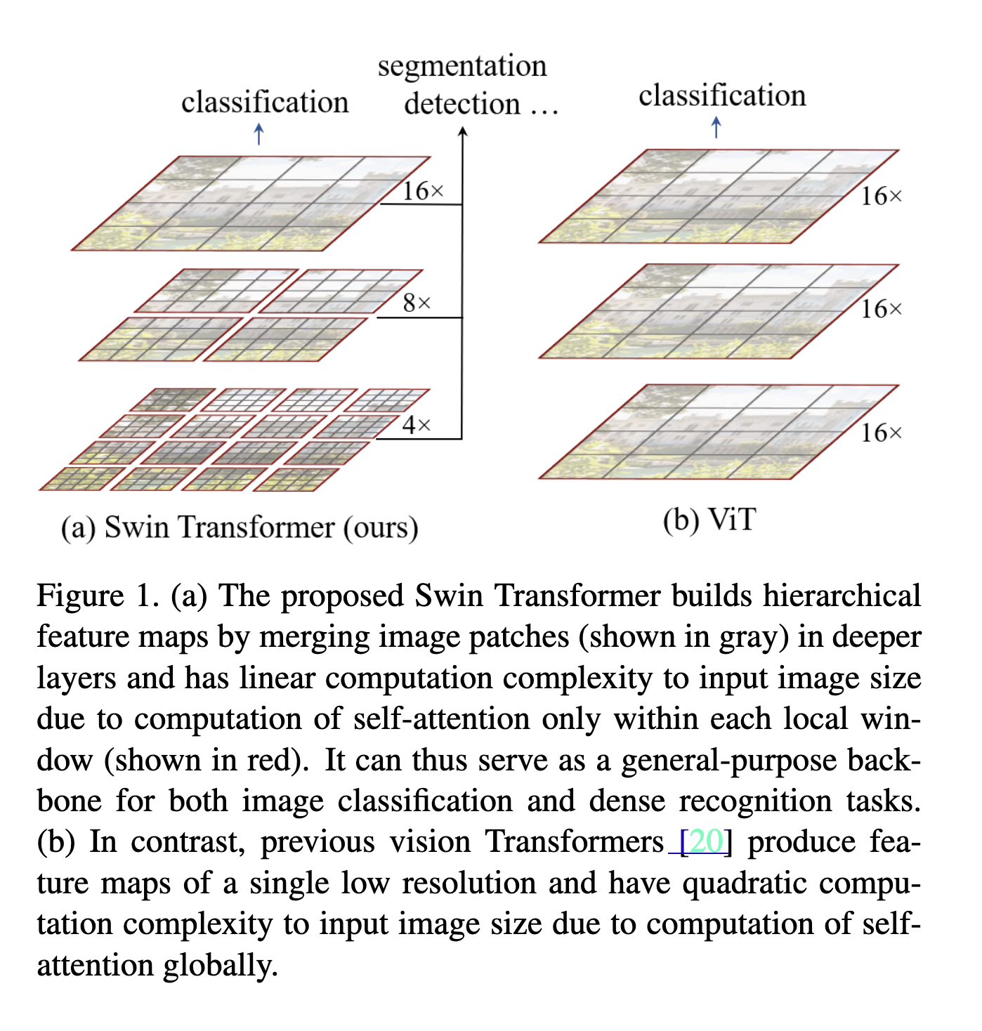
s illustrated in Figure 1(a), Swin Transformer constructs a hierarchical representation by starting from small-sized patches (outlined in gray) and gradually merging neighboring patches in deeper Transformer layers.
Figure 1(a)에서 보이듯, Swin Transformer는 작은 패치(회색으로 표시)로 시작하여 더 깊은 Transformer 계층에서 인접 패치를 점진적으로 병합하며 계층적 표현을 구축한다.
With these hierarchical feature maps, the Swin Transformer model can conveniently leverage advanced techniques for dense prediction such as feature pyramid networks (FPN) [42] or U-Net [51].
이 계층적 특성 맵 덕분에 Swin Transformer는 FPN [42], U-Net [51]과 같은 고급 조밀 예측 기법을 손쉽게 활용할 수 있다.
The linear computational complexity is achieved by computing self-attention locally within non-overlapping windows that partition an image (outlined in red).
선형 복잡도는 이미지를 비겹침 윈도우(빨간색으로 표시)로 나누고, 각 윈도우 내부에서만 self-attention을 계산하는 방식으로 달성된다.
The number of patches in each window is fixed, and thus the complexity becomes linear to image size.
각 윈도우에 포함되는 패치 수가 고정되어 있기 때문에 계산 복잡도는 이미지 크기에 대해 선형이 된다.
These merits make Swin Transformer suitable as a general-purpose backbone for various vision tasks,
이러한 장점들은 Swin Transformer를 다양한 비전 작업에 적합한 범용 백본으로 만든다.
in contrast to previous Transformer based architectures [20] which produce feature maps of a single resolution and have quadratic complexity.
이는 단일 해상도의 특성 맵만 생성하고 이차 복잡도를 가진 기존 Transformer 기반 구조 [20]와는 대조적이다.
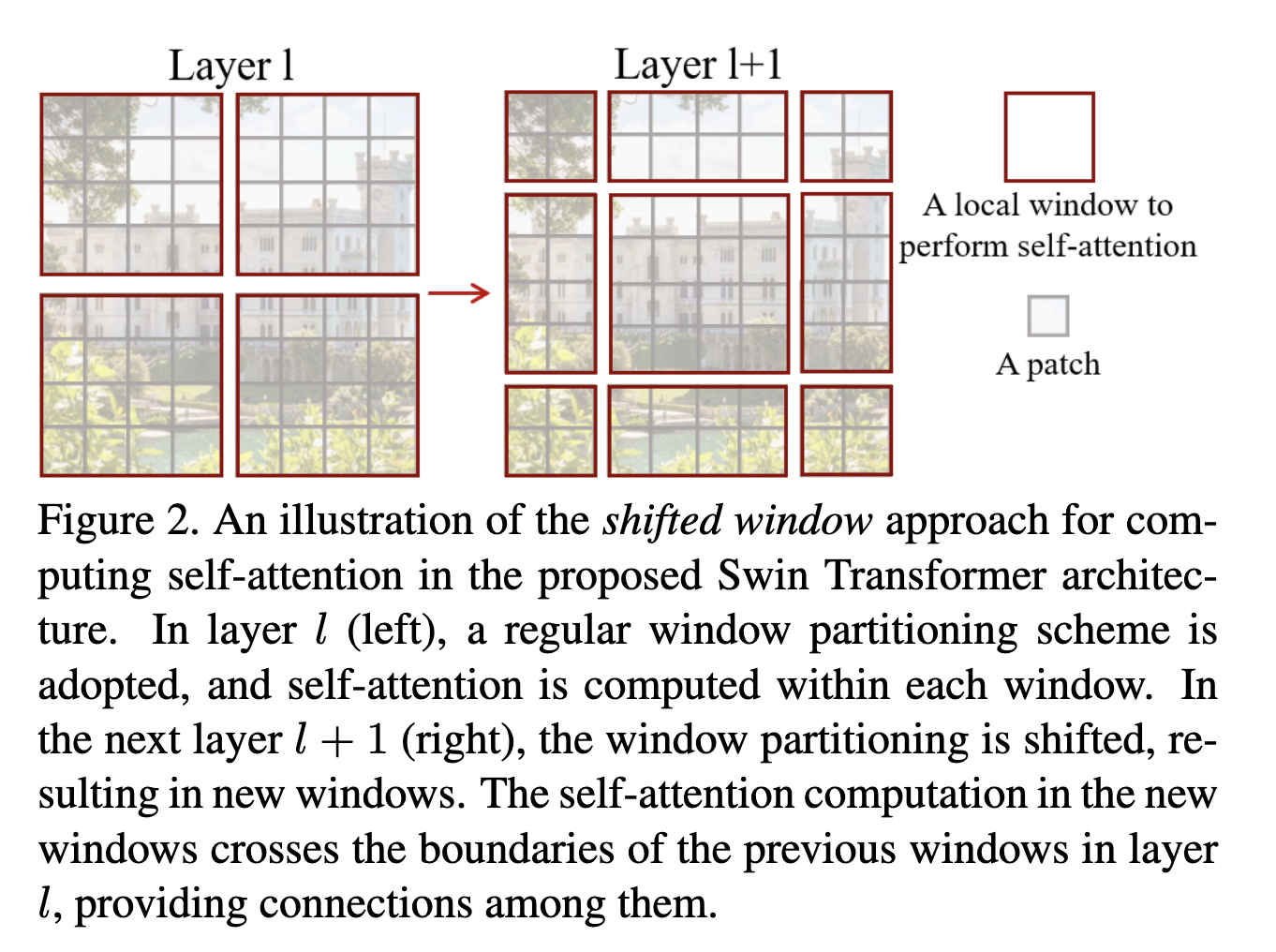
A key design element of Swin Transformer is its shift of the window partition between consecutive self-attention layers, as illustrated in Figure 2.
Swin Transformer의 핵심 설계 요소는 Figure 2에 나타난 것처럼 연속된 self-attention 레이어 간에 윈도우 분할을 이동(shift)시키는 방식이다.
The shifted windows bridge the windows of the preceding layer, providing connections among them that significantly enhance modeling power (see Table 4).
Shifted window는 이전 레이어의 윈도우들을 서로 연결해주며, 이를 통해 모델링 능력을 크게 향상시킨다(Table 4 참조).
This strategy is also efficient in regards to real-world latency: all query patches within a window share the same key set, which facilitates memory access in hardware.
이 전략은 실제 지연(latency) 측면에서도 효율적이다. 하나의 윈도우 내의 모든 query 패치는 동일한 key 집합을 공유하며, 이는 하드웨어에서 메모리 접근을 용이하게 한다.
In contrast, earlier sliding window based self-attention approaches [33, 50] suffer from low latency on general hardware due to different key sets for different query pixels.
반면, 기존의 슬라이딩 윈도 기반 self-attention 방식 [33, 50]은 각 query 픽셀마다 key 집합이 달라 일반 하드웨어에서 지연이 커지는 문제가 있다.
Our experiments show that the proposed shifted window approach has much lower latency than the sliding window method, yet is similar in modeling power (see Tables 5 and 6).
실험 결과, 제안된 shifted window 방식은 슬라이딩 윈도 방식보다 지연이 훨씬 낮으면서도 모델링 성능은 유사함을 확인했다(Tables 5, 6 참조).
The shifted window approach also proves beneficial for all-MLP architectures [61].
또한 shifted window 방식은 순수 MLP 기반 아키텍처(all-MLP) [61]에도 유용한 것으로 확인되었다.
The proposed Swin Transformer achieves strong performance on the recognition tasks of image classification, object detection and semantic segmentation.
제안된 Swin Transformer는 이미지 분류, 객체 탐지, 시맨틱 세그멘테이션과 같은 인식 작업에서 강력한 성능을 보인다.
It outperforms the ViT / DeiT [20, 63] and ResNe(X)t models [30, 70] significantly with similar latency on the three tasks.
세 작업에서 유사한 수준의 지연(latency)을 유지하면서 ViT/DeiT [20, 63] 및 ResNe(X)t [30, 70] 모델을 크게 능가한다.
Its 58.7 box AP and 51.1 mask AP on the COCO test-dev set surpass the previous state-of-the-art results by +2.7 box AP (Copy-paste [26] without external data) and +2.6 mask AP (DetectoRS [46]).
COCO test-dev 기준 box AP 58.7, mask AP 51.1 성능은 이전 SOTA 대비 box AP +2.7(Copy-paste [26], 외부 데이터 없음), mask AP +2.6(DetectoRS [46])을 초과한다.
On ADE20K semantic segmentation, it obtains 53.5 mIoU on the val set, an improvement of +3.2 mIoU over the previous state-of-the-art (SETR [81]).
ADE20K 시맨틱 세그멘테이션에서는 val 기준 53.5 mIoU를 기록하며, 이전 SOTA인 SETR [81] 대비 +3.2 mIoU 향상되었다.
It also achieves a top-1 accuracy of 87.3% on ImageNet-1K image classification.
ImageNet-1K 이미지 분류에서도 Top-1 정확도 87.3%를 달성했다.
It is our belief that a unified architecture across computer vision and natural language processing could benefit both fields,
우리는 컴퓨터 비전과 자연어 처리 전반에서 통합된 아키텍처가 양쪽 분야 모두에 이점을 가져올 것이라고 믿는다.
since it would facilitate joint modeling of visual and textual signals and the modeling knowledge from both domains can be more deeply shared.
이는 시각적·언어적 신호의 공동 모델링을 용이하게 하고, 두 도메인 간 모델링 지식을 더욱 깊게 공유할 수 있게 하기 때문이다.
We hope that Swin Transformer’s strong performance on various vision problems can drive this belief deeper in the community and encourage unified modeling of vision and language signals.
Swin Transformer가 다양한 비전 문제에서 보여준 강력한 성능이 이러한 믿음을 더욱 강화하고, 비전·언어 신호의 통합 모델링을 촉진하기를 기대한다.
2. Related Work
CNN and variants
CNN and variants CNNs serve as the standard network model throughout computer vision.
CNN과 그 변형들은 컴퓨터 비전 전반에서 표준 네트워크 모델로 사용되어 왔다.
While the CNN has existed for several decades [40], it was not until the introduction of AlexNet [39] that the CNN took off and became mainstream.
CNN은 수십 년 전부터 존재해왔지만[40], AlexNet [39]이 등장하기 전까지는 주요 모델로 자리 잡지 못했다.
Since then, deeper and more effective convolutional neural architectures have been proposed to further propel the deep learning wave in computer vision, e.g., VGG [52], GoogleNet [57], ResNet [30], DenseNet [34], HRNet [65], and EfficientNet [58].
그 이후 VGG [52], GoogleNet [57], ResNet [30], DenseNet [34], HRNet [65], EfficientNet [58] 등 더욱 깊고 효율적인 합성곱 기반 신경망 구조들이 등장하며, 컴퓨터 비전에서 딥러닝의 발전을 가속시켰다.
In addition to these architectural advances, there has also been much work on improving individual convolution layers, such as depthwise convolution [70] and deformable convolution [18, 84].
이러한 아키텍처적 발전 외에도 depthwise convolution [70], deformable convolution [18, 84]과 같은 개별 합성곱 연산을 개선하려는 연구도 활발히 진행되었다.
While the CNN and its variants are still the primary backbone architectures for computer vision applications,
CNN과 그 변형들이 여전히 컴퓨터 비전 응용에서 주된 백본 구조이지만,
we highlight the strong potential of Transformer-like architectures for unified modeling between vision and language.
우리는 Transformer 계열 아키텍처가 비전과 언어를 통합적으로 모델링하는 데 큰 잠재력을 가지고 있음을 강조한다.
Our work achieves strong performance on several basic visual recognition tasks, and we hope it will contribute to a modeling shift.
우리의 연구는 여러 기본적인 시각 인식 작업에서 높은 성능을 보였으며, 이를 바탕으로 모델링 패러다임의 전환에도 기여하길 기대한다.
Self-attention based backbone architectures
Self-attention 기반 백본 아키텍처
Also inspired by the success of self-attention layers and Transformer architectures in the NLP field, some works employ self-attention layers to replace some or all of the spatial convolution layers in the popular ResNet [33, 50, 80].
NLP 분야에서 self-attention과 Transformer 아키텍처가 성공한 것에 영감을 받아, 일부 연구는 ResNet [33, 50, 80]의 공간적 합성곱 레이어 일부 또는 전부를 self-attention 레이어로 대체하였다.
In these works, the self-attention is computed within a local window of each pixel to expedite optimization [33], and they achieve slightly better accuracy/FLOPs trade-offs than the counterpart ResNet architecture.
이 연구들에서는 최적화를 빠르게 하기 위해 각 픽셀 주변의 로컬 윈도우 내에서 self-attention을 계산하며[33], 그 결과 대응되는 ResNet 아키텍처보다 약간 더 나은 정확도/FLOPs 균형을 달성한다.
However, their costly memory access causes their actual latency to be significantly larger than that of the convolutional networks [33].
그러나 비싼 메모리 접근 비용 때문에 실제 지연(latency)은 합성곱 신경망보다 훨씬 크다는 문제가 있다[33].
Instead of using sliding windows, we propose to shift windows between consecutive layers, which allows for a more efficient implementation in general hardware.
슬라이딩 윈도 방식을 사용하는 대신, 우리는 레이어 간 윈도우를 이동(shift)시키는 방식을 제안하며, 이는 일반 하드웨어에서 훨씬 효율적인 구현을 가능하게 한다.
Self-attention/Transformers to complement CNNs
CNN을 보완하기 위한 Self-attention/Transformer 기반 접근
Another line of work is to augment a standard CNN architecture with self-attention layers or Transformers.
또 다른 연구 방향은 기존 CNN 구조에 self-attention 레이어나 Transformer를 추가하여 보완하는 것이다.
The self-attention layers can complement backbones [67, 7, 3, 71, 23, 74, 55] or head networks [32, 27] by providing the capability to encode distant dependencies or heterogeneous interactions.
Self-attention 레이어는 원거리 의존성이나 복잡한 상호작용을 인코딩하는 능력을 제공함으로써 백본[67, 7, 3, 71, 23, 74, 55] 또는 헤드 네트워크[32, 27]를 보완할 수 있다.
More recently, the encoder-decoder design in Transformer has been applied for the object detection and instance segmentation tasks [8, 13, 85, 56].
최근에는 Transformer의 인코더–디코더 구조가 객체 탐지 및 인스턴스 세그멘테이션 작업[8, 13, 85, 56]에 적용되었다.
Our work explores the adaptation of Transformers for basic visual feature extraction and is complementary to these works.
우리 연구는 기본적인 시각 특징 추출을 위해 Transformer를 어떻게 적응시킬 수 있는지 탐구하며, 이러한 기존 연구들과 상호 보완적인 역할을 한다.
Transformer based vision backbones
Most related to our work is the Vision Transformer (ViT) [20] and its follow-ups [63, 72, 15, 28, 66].
Transformer 기반 비전 백본 중 우리 연구와 가장 밀접한 것은 Vision Transformer(ViT) [20]와 그 후속 연구들 [63, 72, 15, 28, 66]이다.
The pioneering work of ViT directly applies a Transformer architecture on non-overlapping medium-sized image patches for image classification.
선구적 연구인 ViT는 겹치지 않는 중간 크기의 이미지 패치에 Transformer 아키텍처를 직접 적용하여 이미지 분류를 수행한다.
It achieves an impressive speed-accuracy tradeoff on image classification compared to convolutional networks.
ViT는 합성곱 신경망과 비교했을 때 이미지 분류에서 뛰어난 속도–정확도 균형을 달성한다.
While ViT requires large-scale training datasets (i.e., JFT-300M) to perform well, DeiT [63] introduces several training strategies that allow ViT to also be effective using the smaller ImageNet-1K dataset.
하지만 ViT는 성능을 내기 위해 JFT-300M 같은 대규모 학습 데이터셋이 필요하며, DeiT [63]는 ViT가 상대적으로 작은 ImageNet-1K 데이터셋에서도 효과적으로 학습될 수 있도록 여러 훈련 전략을 도입했다.
The results of ViT on image classification are encouraging, but its architecture is unsuitable for use as a general-purpose backbone network on dense vision tasks or when the input image resolution is high, due to its low-resolution feature maps and the quadratic increase in complexity with image size.
ViT는 이미지 분류에서 고무적인 성과를 보였지만, 낮은 해상도의 특성 맵과 이미지 크기에 대한 이차적 복잡도 증가 때문에 고해상도 입력이나 조밀(dense)한 비전 작업에서 범용 백본으로 사용하기에는 적합하지 않다.
There are a few works applying ViT models to the dense vision tasks of object detection and semantic segmentation by direct upsampling or deconvolution but with relatively lower performance [2, 81].
직접 업샘플링 또는 디컨볼루션을 통해 ViT를 객체 탐지나 시맨틱 세그멘테이션 같은 조밀한 비전 작업에 적용한 연구도 일부 존재하지만, 상대적으로 성능이 낮다 [2, 81].
Concurrent to our work are some that modify the ViT architecture [72, 15, 28] for better image classification.
우리 연구와 동시에 진행된 몇몇 연구에서는 이미지 분류 성능을 위해 ViT 아키텍처를 수정한 바 있다 [72, 15, 28].
Empirically, we find our Swin Transformer architecture to achieve the best speed-accuracy trade-off among these methods on image classification, even though our work focuses on general-purpose performance rather than specifically on classification.
경험적으로, 비록 본 연구는 분류가 아닌 범용 성능을 목표로 하지만, 이미지 분류 기준에서 Swin Transformer는 이들 방법 중 가장 뛰어난 속도–정확도 균형을 보였다.
Another concurrent work [66] explores a similar line of thinking to build multi-resolution feature maps on Transformers.
또 다른 동시 연구 [66]는 Transformer에서 다중 해상도 특성 맵을 구성하는 유사한 접근을 탐구했다.
Its complexity is still quadratic to image size, while ours is linear and also operates locally which has proven beneficial in modeling the high correlation in visual signals [36, 25, 41].
하지만 해당 연구는 여전히 이미지 크기에 대해 복잡도가 이차적이며, 반면 우리의 방법은 선형 복잡도를 가지며 로컬 방식으로 동작해 시각 신호의 높은 상관관계를 모델링하는 데 효과적임이 입증되었다[36, 25, 41].
Our approach is both efficient and effective, achieving state-of-the-art accuracy on both COCO object detection and ADE20K semantic segmentation.
우리의 접근법은 효율성과 효과성을 모두 갖추고 있으며, COCO 객체 탐지와 ADE20K 시맨틱 세그멘테이션에서 SOTA 성능을 달성했다.
3. Method
3.1. Overall Architecture
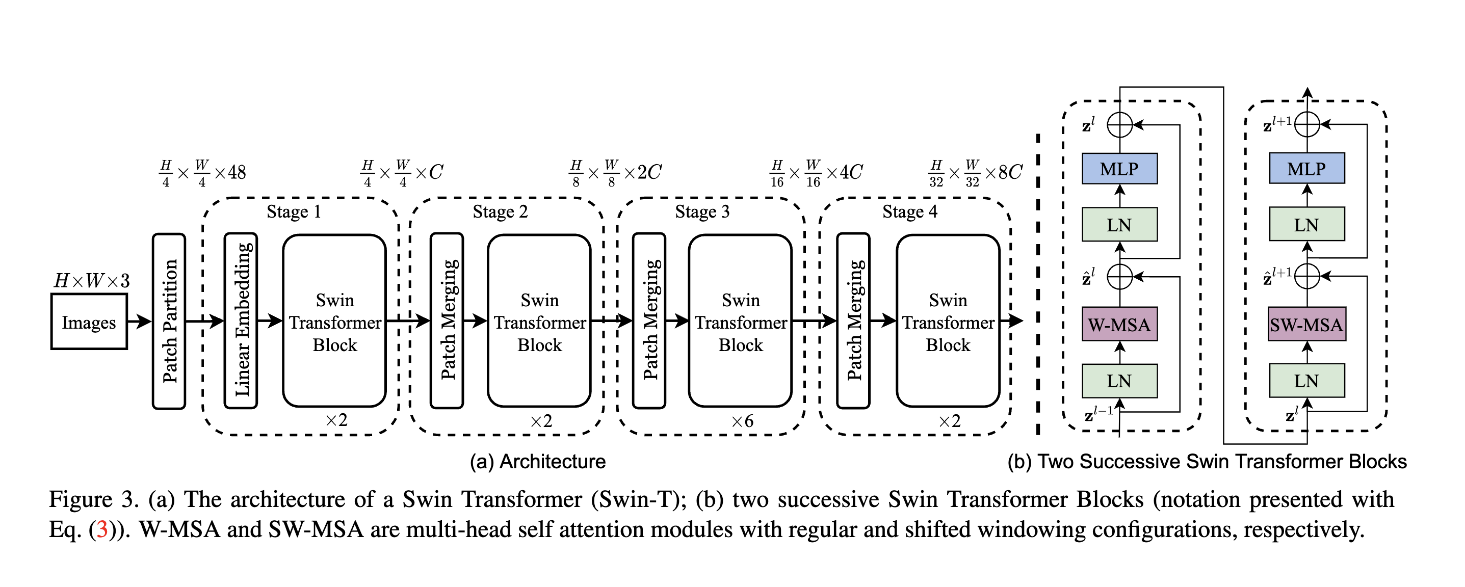
An overview of the Swin Transformer architecture is presented in Figure 3, which illustrates the tiny version (Swin-T).
Figure 3은 Swin Transformer 구조의 개요를 보여주며, tiny 버전(Swin-T)을 예시로 설명한다.
It first splits an input RGB image into non-overlapping patches by a patch splitting module, like ViT.
먼저 입력 RGB 이미지를 ViT와 동일하게 패치 분할 모듈로 겹치지 않는 패치들로 분할한다.
Each patch is treated as a “token” and its feature is set as a concatenation of the raw pixel RGB values.
각 패치는 하나의 “토큰”으로 간주되며, 그 특성(feature)은 해당 패치의 원본 픽셀 RGB 값을 단순 연결한 벡터로 설정된다.
In our implementation, we use a patch size of 4 × 4 and thus the feature dimension of each patch is 4 × 4 × 3 = 48.
본 구현에서는 패치 크기를 4×4로 사용하며, 각 패치의 feature 차원은 4×4×3 = 48이다.
A linear embedding layer is applied on this raw-valued feature to project it to an arbitrary dimension (denoted as C).
이 원시 값 기반 feature에 대해 임의 차원(C)으로 투영(projection)하기 위해 선형 임베딩 레이어가 적용된다.
Several Transformer blocks with modified self-attention computation (Swin Transformer blocks) are applied on these patch tokens.
이 패치 토큰들에 대해 수정된 self-attention 계산을 사용하는 여러 Transformer 블록(Swin Transformer 블록)이 적용된다.
The Transformer blocks maintain the number of tokens (H/4 × W/4), and together with the linear embedding are referred to as “Stage 1”.
이 Transformer 블록들은 토큰 수(H/4 × W/4)를 유지하며, 선형 임베딩과 함께 이 전체 구성은 “Stage 1”로 정의된다.
To produce a hierarchical representation, the number of tokens is reduced by patch merging layers as the network gets deeper.
계층적 표현을 생성하기 위해 네트워크가 깊어질수록 패치 병합(patch merging) 레이어를 통해 토큰 수가 감소된다.
The first patch merging layer concatenates the features of each group of 2 × 2 neighboring patches, and applies a linear layer on the 4C-dimensional concatenated features.
첫 번째 패치 병합 레이어는 2×2 이웃 패치들의 feature를 연결(concatenate)하여 4C 차원 벡터를 만들고, 여기에 선형 레이어를 적용한다.
This reduces the number of tokens by a multiple of 2 × 2 = 4 (2× downsampling of resolution), and the output dimension is set to 2C.
이를 통해 토큰 수는 2×2=4배 줄어들며(해상도 2배 다운샘플링), 출력 feature 차원은 2C로 설정된다.
Swin Transformer blocks are applied afterwards for feature transformation, with the resolution kept at H/8 × W/8.
이후 Swin Transformer 블록이 적용되어 feature 변환을 수행하며, 해상도는 H/8 × W/8로 유지된다.
This first block of patch merging and feature transformation is denoted as “Stage 2”.
이 첫 번째 패치 병합 + feature 변환 블록이 “Stage 2”에 해당한다.
The procedure is repeated twice, as “Stage 3” and “Stage 4”, with output resolutions of H/16 × W/16 and H/32 × W/32, respectively.
이 과정은 이후 두 번 반복되어 각각 H/16 × W/16, H/32 × W/32 해상도를 갖는 “Stage 3”와 “Stage 4”를 형성한다.
These stages jointly produce a hierarchical representation, with the same feature map resolutions as those of typical convolutional networks, e.g., VGG [52] and ResNet [30].
이 모든 스테이지는 VGG [52], ResNet [30]과 같은 전통적인 CNN 백본이 생성하는 것과 동일한 해상도의 계층적 feature map을 생성한다.
As a result, the proposed architecture can conveniently replace the backbone networks in existing methods for various vision tasks.
그 결과 제안된 아키텍처는 다양한 비전 작업에서 기존 CNN 백본을 쉽게 대체할 수 있다.
Swin Transformer block
Swin Transformer is built by replacing the standard multi-head self attention (MSA) module in a Transformer block by a module based on shifted windows (described in Section 3.2), with other layers kept the same.
Swin Transformer 블록은 기존 Transformer 블록의 표준 MSA(Multi-Head Self-Attention) 모듈을 shifted window 기반 모듈(Section 3.2 설명)로 대체하고, 나머지 레이어 구조는 그대로 유지하여 구성된다.
As illustrated in Figure 3(b), a Swin Transformer block consists of a shifted window based MSA module, followed by a 2-layer MLP with GELU nonlinearity in between.
Figure 3(b)에 나타난 것처럼, Swin Transformer 블록은 shifted window 기반 MSA 모듈과 그 뒤에 GELU 비선형성을 포함한 2층 MLP로 이루어진다.
A LayerNorm (LN) layer is applied before each MSA module and each MLP, and a residual connection is applied after each module.
각 MSA 모듈과 MLP 앞에는 LayerNorm(LN)이 적용되며, 각 모듈 뒤에는 잔차 연결(residual connection)이 적용된다.
3.2. Shifted Window based Self-Attention
The standard Transformer architecture [64] and its adaptation for image classification [20] both conduct global self-attention, where the relationships between a token and all other tokens are computed.
기존 Transformer 아키텍처 [64]와 이를 이미지 분류에 적용한 ViT [20]은 모두 전역 self-attention을 수행하는데, 이 방식은 한 토큰과 모든 다른 토큰 간의 관계를 계산한다.
The global computation leads to quadratic complexity with respect to the number of tokens, making it unsuitable for many vision problems requiring an immense set of tokens for dense prediction or to represent a high-resolution image.
전역 연산은 토큰 개수에 대해 이차적 복잡도를 가지므로, 고해상도 이미지나 조밀한 예측을 위해 매우 많은 토큰이 필요한 비전 문제에는 적합하지 않다.
Self-attention in non-overlapped windows
For efficient modeling, we propose to compute self-attention within local windows.
효율적인 모델링을 위해 우리는 로컬 윈도우 내부에서 self-attention을 계산하는 방법을 제안한다.
The windows are arranged to evenly partition the image in a non-overlapping manner.
이 윈도우들은 이미지 전체를 균등하게, 겹치지 않게 분할하도록 구성된다.
Supposing each window contains M × M patches, the computational complexity of a global MSA module and a window-based one where the former is quadratic to patch number hw, and the latter is linear when M is fixed (set to 7 by default).
각 윈도우가 M×M 패치를 포함한다고 할 때, 전역 MSA의 복잡도는 전체 패치 수인 h·w에 대해 이차적이며, 윈도우 기반 MSA의 복잡도는 M이 고정되면 선형이 된다(기본값 M = 7).
Global self-attention computation is generally unaffordable for a large hw, while the window based self-attention is scalable.
전역 self-attention은 h·w가 큰 경우 계산이 사실상 불가능하지만, 윈도우 기반 self-attention은 확장 가능하다.
Shifted window partitioning in successive blocks
The window-based self-attention module lacks connections across windows, which limits its modeling power.
윈도우 기반 self-attention은 윈도우 간 연결이 없어 모델링 능력이 제한된다.
To introduce cross-window connections while maintaining the efficient computation of non-overlapping windows, we propose a shifted window partitioning approach which alternates between two partitioning configurations in consecutive Swin Transformer blocks.
겹치지 않는 윈도우의 효율성을 유지하면서 윈도우 간 연결을 도입하기 위해, 우리는 Swin Transformer 블록마다 서로 다른 두 종류의 윈도우 분할 방식을 번갈아 사용하는 ‘shifted window partitioning’을 제안한다.
As illustrated in Figure 2, the first module uses a regular window partitioning strategy which starts from the top-left pixel, and the 8×8 feature map is evenly partitioned into 2×2 windows of size 4×4 (M = 4).
Figure 2에서 보듯, 첫 번째 모듈은 좌상단 픽셀에서 시작하는 일반적인 윈도우 분할 방식을 사용하며, 8×8 feature map은 4×4 크기의 2×2 윈도우로 균등하게 분할된다(M=4).
Then, the next module adopts a windowing configuration that is shifted from that of the preceding layer, by displacing the windows by (⌊M/2⌋, ⌊M/2⌋) pixels from the regularly partitioned windows.
다음 모듈은 이전 레이어의 윈도우 분할에서 (⌊M/2⌋, ⌊M/2⌋) 만큼 이동한 shifted window 구성을 사용한다.
Computation flow of consecutive Swin Transformer blocks
With the shifted window partitioning approach, consecutive Swin Transformer blocks are computed as
shifted window 분할 방식을 사용하면 연속된 Swin Transformer 블록은 아래와 같이 계산된다:
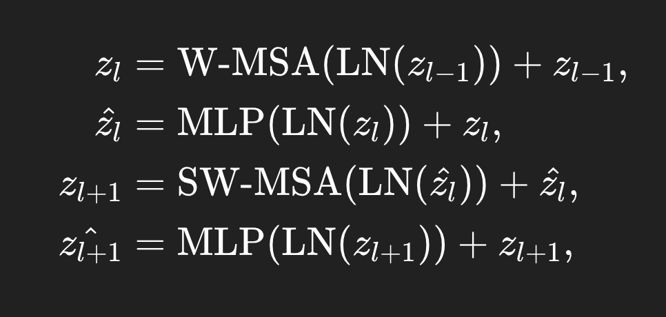
where zl^\hat{z_l}zl^ and zlz_lzl denote the output features of the (S)W-MSA module and the MLP module for block l, respectively;
여기서 zl^\hat{z_l}zl^과 zlz_lzl은 각각 블록 lll의 (S)W-MSA 모듈 출력과 MLP 모듈 출력을 의미한다.
W-MSA and SW-MSA denote window based multi-head self-attention using regular and shifted window partitioning configurations, respectively.
W-MSA는 일반 윈도우 분할 기반 self-attention, SW-MSA는 shifted window 기반 self-attention을 의미한다.
The shifted window partitioning approach introduces connections between neighboring non-overlapping windows in the previous layer and is found to be effective in image classification, object detection, and semantic segmentation, as shown in Table 4.
shifted window 분할 방식은 이전 레이어의 이웃하는 비겹침 윈도우들 간 연결을 생성하며, Table 4에서 보이듯 이미지 분류, 객체 탐지, 시맨틱 세그멘테이션에서 효과적임이 확인되었다.
Efficient batch computation for shifted configuration
Efficient batch computation for shifted configuration
An issue with shifted window partitioning is that it will result in more windows, from ⌈h/M⌉ × ⌈w/M⌉ to (⌈h/M⌉ + 1) × (⌈w/M⌉ + 1) in the shifted configuration, and some of the windows will be smaller than M × M.
Shifted window 분할의 문제점은, 기존 ⌈h/M⌉ × ⌈w/M⌉ 윈도우보다 더 많은 윈도우가 생성되며 shifted 구성에서는 (⌈h/M⌉ + 1) × (⌈w/M⌉ + 1) 으로 증가하고, 일부 윈도우는 크기가 M×M보다 작아진다는 점이다.
A naive solution is to pad the smaller windows to a size of M × M and mask out the padded values when computing attention.
단순한 해결책으로는 작은 윈도우를 M×M 크기로 패딩한 후, attention 계산 시 패딩된 값을 마스킹하는 방법이 있다.
When the number of windows in regular partitioning is small, e.g. 2 × 2, the increased computation with this naive solution is considerable (2 × 2 → 3 × 3, which is 2.25 times greater).
하지만 일반 분할에서 윈도우 수가 2×2처럼 적을 경우, 이 단순 방식은 계산량이 크게 증가하며(2×2 → 3×3으로 2.25배 증가) 비효율적이다.
Here, we propose a more efficient batch computation approach by cyclic-shifting toward the top-left direction, as illustrated in Figure 4.
이에 우리는 Figure 4에서 보이듯, feature map을 좌상단 방향으로 cyclic shift하여 더 효율적인 배치(batch) 연산 방식을 제안한다.
After this shift, a batched window may be composed of several sub-windows that are not adjacent in the feature map, so a masking mechanism is employed to limit self-attention computation to within each sub-window.
이 cyclic shift 이후에는 하나의 배치된 윈도우가 서로 인접하지 않은 여러 sub-window로 구성될 수 있다. 따라서 self-attention 계산을 각 sub-window 내부로 제한하기 위해 마스킹 메커니즘을 적용한다.
With the cyclic-shift, the number of batched windows remains the same as that of regular window partitioning, and thus is also efficient.
Cyclic shift를 사용하면 배치된 윈도우 수가 기존 regular window 분할과 동일하게 유지되므로 계산 효율성이 높아진다.
The low latency of this approach is shown in Table 5.
이 방식의 낮은 지연(latency)은 Table 5에서 확인할 수 있다.
Relative position bias
In computing self-attention, we follow [49, 1, 32, 33] by including a relative position bias B ∈ ℝ^(M²×M²) to each head in computing similarity:
Self-attention 계산 시 우리는 [49, 1, 32, 33]을 따라, 각 head의 similarity 계산에 상대적 위치 편향(relative position bias) B ∈ ℝ^(M²×M²)을 포함한다:
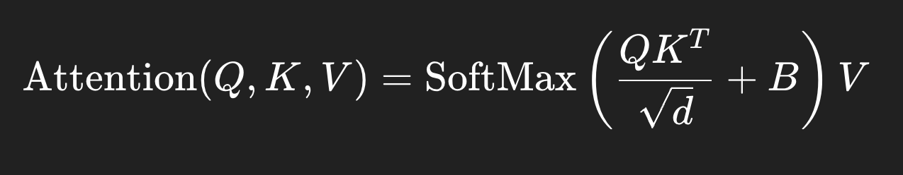
Attention(Q,K,V)=SoftMax(d
QKT+B)V
where Q, K, V ∈ ℝ^(M²×d) are the query, key and value matrices; d is the query/key dimension, and M² is the number of patches in a window.
여기서 Q, K, V ∈ ℝ^(M²×d)은 query, key, value 행렬이며, d는 query/key의 차원이고, M²은 한 윈도우에 포함된 패치 수이다.
Since the relative position along each axis lies in the range [−M + 1, M − 1], we parameterize a smaller-sized bias matrix B^∈R(2M−1)×(2M−1)\hat{B} ∈ ℝ^{(2M−1)×(2M−1)}B^∈R(2M−1)×(2M−1), and values in B are taken from B^\hat{B}B^.
각 축에서의 상대적 위치 값이 [−M+1, M−1] 범위를 가지므로, 더 작은 크기의 편향 행렬 B^∈R(2M−1)×(2M−1)\hat{B} ∈ ℝ^{(2M−1)×(2M−1)}B^∈R(2M−1)×(2M−1)를 학습 파라미터로 사용하고, 실제 B의 값은 B^\hat{B}B^에서 가져와 구성한다.
We observe significant improvements over counterparts without this bias term or that use absolute position embedding, as shown in Table 4.
Table 4에서 보이듯, 상대적 위치 편향을 사용하지 않거나 절대적 위치 임베딩을 사용하는 모델들보다 성능이 크게 향상되는 것을 확인했다.
Further adding absolute position embedding to the input as in [20] drops performance slightly, thus it is not adopted in our implementation.
또한 [20]처럼 입력에 절대 위치 임베딩을 추가하면 성능이 다소 감소하여, 본 구현에서는 사용하지 않는다.
The learnt relative position bias in pre-training can be also used to initialize a model for fine-tuning with a different window size through bi-cubic interpolation [20, 63].
사전 학습에서 학습된 상대 위치 편향은, 다른 윈도우 크기로 미세 조정(fine-tuning)할 때도 bi-cubic interpolation [20, 63]을 통해 초기화 값으로 사용할 수 있다.
3.3. Architecture Variants
We build our base model, called Swin-B, to have model size and computation complexity similar to ViT-B/DeiT-B.
우리는 기본 모델인 Swin-B를 ViT-B/DeiT-B와 비슷한 모델 크기와 연산 복잡도를 갖도록 설계했다.
We also introduce Swin-T, Swin-S and Swin-L, which are versions of about 0.25×, 0.5× and 2× the model size and computational complexity, respectively.
또한 Swin-T, Swin-S, Swin-L을 제안하며, 각각 모델 크기와 연산량이 약 0.25배, 0.5배, 2배에 해당하는 버전이다.
Note that the complexity of Swin-T and Swin-S are similar to those of ResNet-50 (DeiT-S) and ResNet-101, respectively.
Swin-T의 복잡도는 ResNet-50(또는 DeiT-S)와 비슷하며, Swin-S는 ResNet-101과 유사한 복잡도를 가진다.
The window size is set to M = 7 by default.
기본 윈도우 크기는 M = 7로 설정한다.
The query dimension of each head is d = 32, and the expansion layer of each MLP is α = 4, for all experiments.
모든 실험에서 각 head의 query 차원 d는 32이며, 각 MLP의 확장 계수 α는 4를 사용한다.
Architecture Hyper-parameters
The architecture hyper-parameters of these model variants are:
다음은 각 Swin 모델 버전의 아키텍처 하이퍼파라미터이다:
- Swin-T: C = 96, layer numbers = {2, 2, 6, 2}
- Swin-S: C = 96, layer numbers = {2, 2, 18, 2}
- Swin-B: C = 128, layer numbers = {2, 2, 18, 2}
- Swin-L: C = 192, layer numbers = {2, 2, 18, 2}
where C is the channel number of the hidden layers in the first stage.
여기서 C는 첫 번째 스테이지의 hidden layer 채널 수를 의미한다.
The model size, theoretical computational complexity (FLOPs), and throughput of the model variants for ImageNet image classification are listed in Table 1.
ImageNet 이미지 분류 기준에서 모델 크기, 이론적 연산량(FLOPs), 처리량(throughput)은 Table 1에 정리되어 있다.
4. Experiments
We conduct experiments on ImageNet-1K image classification [19], COCO object detection [43], and ADE20K semantic segmentation [83].
우리는 ImageNet-1K 이미지 분류 [19], COCO 객체 탐지 [43], ADE20K 시맨틱 세그멘테이션 [83]에서 실험을 수행했다.
In the following, we first compare the proposed Swin Transformer architecture with the previous state-of-the-arts on the three tasks.
이후 섹션에서는 세 작업에서 제안한 Swin Transformer와 기존 SOTA 모델들을 비교한다.
Then, we ablate the important design elements of Swin Transformer.
그 다음 Swin Transformer의 주요 설계 요소들에 대한 ablation 연구를 수행한다.
4.1. Image Classification on ImageNet-1K
Settings
For image classification, we benchmark the proposed Swin Transformer on ImageNet-1K [19], which contains 1.28M training images and 50K validation images from 1,000 classes.
이미지 분류 실험에서는 Swin Transformer를 ImageNet-1K [19]에서 벤치마크한다. 이 데이터셋은 1,000개 클래스에 대해 128만 개의 학습 이미지와 5만 개의 검증 이미지를 포함한다.
The top-1 accuracy on a single crop is reported.
단일 crop 기준의 top-1 정확도를 보고한다.
We consider two training settings:
두 가지 훈련 설정을 고려한다:
Regular ImageNet-1K training
This setting mostly follows [63].
이 설정은 주로 [63]의 설정을 따른다.
We employ an AdamW [37] optimizer for 300 epochs using a cosine decay learning rate scheduler and 20 epochs of linear warm-up.
300 epoch 동안 AdamW [37] 옵티마이저를 사용하며, cosine decay 학습률 스케줄러와 20 epoch의 linear warm-up을 적용한다.
A batch size of 1024, an initial learning rate of 0.001, and a weight decay of 0.05 are used.
배치 크기는 1024, 초기 학습률은 0.001, weight decay는 0.05를 사용한다.
We include most of the augmentation and regularization strategies of [63] in training, except for repeated augmentation [31] and EMA [45], which do not enhance performance.
훈련에는 [63]의 증강 및 정규화 기법 대부분을 포함하되, repeated augmentation [31]과 EMA [45]는 성능을 높이지 않아 제외했다.
Note that this is contrary to [63] where repeated augmentation is crucial to stabilize the training of ViT.
이는 ViT 학습 안정화에 repeated augmentation이 필수적이던 [63]의 결과와는 대조된다.
Pre-training on ImageNet-22K and fine-tuning on ImageNet-1K
We also pre-train on the larger ImageNet-22K dataset, which contains 14.2 million images and 22K classes.
또한 1,420만 개 이미지와 22,000개 클래스를 포함한 더 큰 데이터셋인 ImageNet-22K에서 사전 학습을 수행한다.
We employ an AdamW optimizer for 90 epochs using a linear decay learning rate scheduler with a 5-epoch linear warm-up.
사전 학습에서는 AdamW 옵티마이저를 사용해 90 epoch 동안 훈련하며, 5 epoch의 linear warm-up 후 linear decay 학습률 스케줄러를 적용한다.
A batch size of 4096, an initial learning rate of 0.001, and a weight decay of 0.01 are used.
배치 크기는 4096, 초기 학습률은 0.001, weight decay는 0.01을 사용한다.
In ImageNet-1K fine-tuning, we train the models for 30 epochs with a batch size of 1024, a constant learning rate of 10⁻⁵, and a weight decay of 10⁻⁸.
ImageNet-1K에서의 fine-tuning은 30 epoch 동안 수행하며, 배치 크기는 1024, 학습률은 10⁻⁵로 고정, weight decay는 10⁻⁸로 설정한다.
Results with regular ImageNet-1K training
Table 1(a) presents comparisons to other backbones, including both Transformer-based and ConvNet-based, using regular ImageNet-1K training.
Table 1(a)는 ImageNet-1K 일반 학습 설정에서 Transformer 기반 및 ConvNet 기반 백본들과 Swin Transformer를 비교한 결과를 보여준다.
Compared to the previous state-of-the-art Transformer-based architecture, i.e. DeiT [63], Swin Transformers noticeably surpass the counterpart DeiT architectures with similar complexities:
이전 SOTA Transformer 기반 구조인 DeiT [63]와 비교하면, Swin Transformer는 유사한 복잡도에서 명확히 더 높은 성능을 보인다:
- *Swin-T (81.3%)는 DeiT-S (79.8%)보다 +1.5% 향상** (입력 224² 기준)
- *Swin-B (83.3% / 84.5%)는 DeiT-B (81.8% / 83.1%)보다 +1.5% / +1.4% 향상** (입력 224² / 384² 기준)
Compared with the state-of-the-art ConvNets, i.e. RegNet [48] and EfficientNet [58], the Swin Transformer achieves a slightly better speed-accuracy trade-off.
SOTA ConvNet인 RegNet [48] 및 EfficientNet [58]과 비교했을 때 Swin Transformer는 속도–정확도 균형(speed-accuracy trade-off)에서 약간 더 우수한 성능을 보인다.
Noting that while RegNet [48] and EfficientNet [58] are obtained via a thorough architecture search, the proposed Swin Transformer is adapted from the standard Transformer and has strong potential for further improvement.
RegNet과 EfficientNet이 광범위한 아키텍처 탐색을 통해 설계된 반면, Swin Transformer는 표준 Transformer에서 변형된 구조임에도 불구하고 이 정도 성능을 내며, 추가 개선 가능성이 크다는 점은 주목할 만하다.
Results with ImageNet-22K pre-training
We also pre-train the larger-capacity Swin-B and Swin-L on ImageNet-22K.
우리는 더 큰 모델인 Swin-B와 Swin-L을 ImageNet-22K에서 사전 학습하였다.
Results fine-tuned on ImageNet-1K image classification are shown in Table 1(b).
ImageNet-1K에서 파인튜닝한 결과는 Table 1(b)에 제시되어 있다.
For Swin-B, the ImageNet-22K pre-training brings 1.8%∼1.9% gains over training on ImageNet-1K from scratch.
Swin-B 모델은 ImageNet-22K 사전 학습을 통해 ImageNet-1K를 처음부터 학습하는 경우보다 1.8%~1.9% 성능 향상을 얻는다.
Compared with the previous best results for ImageNet-22K pre-training, our models achieve significantly better speed-accuracy trade-offs:
이전 ImageNet-22K 사전 학습 기반 SOTA 모델들과 비교했을 때, Swin 모델은 속도–정확도 균형에서 크게 개선된 성능을 보인다:
- Swin-B는
- top-1 accuracy 86.4% 달성,
- 이는 유사한 추론 처리량(inference throughput) 대비 ViT보다 2.4% 더 높음
- 처리량: ViT 84.7 vs. Swin-B 85.9 images/sec
- FLOPs: ViT 55.4G vs. Swin-B 47.0G (더 낮음)
The larger Swin-L model achieves 87.3% top-1 accuracy, +0.9% better than that of the Swin-B model.
더 큰 Swin-L 모델은 top-1 accuracy 87.3%를 달성하여, Swin-B보다 +0.9% 더 높은 성능을 보인다.
4.2. Object Detection on COCO
Settings
Object detection and instance segmentation experiments are conducted on COCO 2017, which contains 118K training, 5K validation and 20K test-dev images.
객체 탐지 및 인스턴스 세그멘테이션 실험은 COCO 2017에서 수행되며, 이 데이터셋은 11만 8천 개의 학습 이미지, 5천 개의 검증 이미지, 2만 개의 test-dev 이미지를 포함한다.
An ablation study is performed using the validation set, and a system-level comparison is reported on test-dev.
검증 세트를 활용해 ablation 연구를 수행하고, test-dev에서 시스템 레벨 비교 결과를 보고한다.
For the ablation study, we consider four typical object detection frameworks: Cascade Mask R-CNN [29, 6], ATSS [79], RepPoints v2 [12], and Sparse RCNN [56] in mmdetection [10].
ablation 실험에서는 mmdetection [10] 내의 대표적인 네 가지 객체 탐지 프레임워크인 Cascade Mask R-CNN [29, 6], ATSS [79], RepPoints v2 [12], Sparse R-CNN [56]을 고려한다.
For these four frameworks, we utilize the same settings: multi-scale training [8, 56] (resizing the input such that the shorter side is between 480 and 800 while the longer side is at most 1333), AdamW [44] optimizer (initial learning rate of 0.0001, weight decay of 0.05, and batch size of 16), and 3x schedule (36 epochs).
이 네 프레임워크 모두 다음과 같은 동일 설정을 사용한다:
- Multi-scale training [8, 56]
- 입력의 짧은 변을 480~800 사이로 조정
- 긴 변은 최대 1333
- AdamW [44] optimizer
- 초기 학습률 0.0001
- weight decay 0.05
- 배치 크기 16
- 3x schedule
- 총 36 epochs
For system-level comparison, we adopt an improved HTC [9] (denoted as HTC++) with instaboost [22], stronger multi-scale training [7], 6x schedule (72 epochs), soft-NMS [5], and ImageNet-22K pre-trained model as initialization.
시스템 레벨 비교에서는 다음을 사용한 개선된 HTC [9] (HTC++로 표기)을 적용한다:
- instaboost [22]
- 더 강력한 multi-scale training [7]
- 6x schedule (72 epochs)
- soft-NMS [5]
- ImageNet-22K 사전학습 모델로 초기화
Backbone Comparison
We compare our Swin Transformer to standard ConvNets, i.e. ResNe(X)t, and previous Transformer networks, e.g. DeiT.
우리는 Swin Transformer를 대표적인 ConvNet 백본인 ResNe(X)t 및 기존 Transformer 백본인 DeiT와 비교한다.
The comparisons are conducted by changing only the backbones with other settings unchanged.
비교는 백본만 교체하고 나머지 설정은 동일하게 유지한 상태에서 수행된다.
Note that while Swin Transformer and ResNe(X)t are directly applicable to all the above frameworks because of their hierarchical feature maps,
Swin Transformer와 ResNe(X)t는 계층적(feature hierarchical) 특성 맵을 생성하므로 앞서 언급된 모든 프레임워크에 직접 적용할 수 있지만,
DeiT only produces a single resolution of feature maps and cannot be directly applied.
DeiT는 단일 해상도의 feature map만 생성하기 때문에 직접 적용할 수 없다.
For fair comparison, we follow [81] to construct hierarchical feature maps for DeiT using deconvolution layers.
공정한 비교를 위해, DeiT에는 [81]을 따라 deconvolution 레이어를 사용하여 계층적 feature map을 구성한다.
Comparison to ResNe(X)t
Table 2(a) lists the results of Swin-T and ResNet-50 on the four object detection frameworks.
Table 2(a)는 네 가지 객체 탐지 프레임워크에서 Swin-T와 ResNet-50의 성능을 비교한 결과를 보여준다.
Our Swin-T architecture brings consistent +3.4∼4.2 box AP gains over ResNet-50, with slightly larger model size, FLOPs and latency.
Swin-T는 ResNet-50 대비 꾸준히 +3.4~4.2 box AP 향상을 제공하며, 모델 크기·FLOPs·지연(latency)은 약간 더 크다.
Table 2(b) compares Swin Transformer and ResNe(X)t under different model capacity using Cascade Mask R-CNN.
Table 2(b)는 Cascade Mask R-CNN을 사용하여 Swin Transformer와 ResNe(X)t를 다양한 모델 규모에서 비교한 결과다.
Swin Transformer achieves a high detection accuracy of 51.9 box AP and 45.0 mask AP,
Swin Transformer는 51.9 box AP, 45.0 mask AP라는 높은 탐지 성능을 달성하며,
which are significant gains of +3.6 box AP and +3.3 mask AP over ResNeXt101-64x4d, which has similar model size, FLOPs and latency.
유사한 모델 크기·FLOPs·지연 시간을 가진 ResNeXt101-64x4d 대비
+3.6 box AP, +3.3 mask AP라는 큰 성능 향상을 보인다.
On a higher baseline of 52.3 box AP and 46.0 mask AP using an improved HTC framework, the gains by Swin Transformer are also high, at +4.1 box AP and +3.1 mask AP (see Table 2(c)).
개선된 HTC 프레임워크(기본 성능 52.3 box AP, 46.0 mask AP)를 사용할 때도
Swin Transformer는 +4.1 box AP, +3.1 mask AP라는 큰 폭의 개선을 달성한다(Table 2(c)).
Regarding inference speed, while ResNe(X)t is built by highly optimized Cudnn functions, our architecture is implemented with built-in PyTorch functions that are not all well-optimized.
추론 속도 측면에서는 ResNe(X)t가 고도로 최적화된 CuDNN 함수 기반인 반면,
Swin Transformer는 PyTorch 기본 연산을 사용해 구현되어 모든 연산이 최적화된 상태는 아니다.
A thorough kernel optimization is beyond the scope of this paper.
커널 최적화는 본 논문의 범위를 벗어난다.
Comparison to DeiT
The performance of DeiT-S using the Cascade Mask R-CNN framework is shown in Table 2(b).
Cascade Mask R-CNN 기반의 DeiT-S 성능은 Table 2(b)에 제시되어 있다.
The results of Swin-T are +2.5 box AP and +2.3 mask AP higher than DeiT-S with similar model size (86M vs. 80M) and significantly higher inference speed (15.3 FPS vs. 10.4 FPS).
Swin-T는 DeiT-S 대비 +2.5 box AP, +2.3 mask AP 더 높으며,
모델 크기(86M vs. 80M)는 비슷하지만 추론 속도는 훨씬 빠르다 (15.3 FPS vs. 10.4 FPS).
The lower inference speed of DeiT is mainly due to its quadratic complexity to input image size.
DeiT의 느린 추론 속도는 입력 이미지 크기에 대해 자승(Quadratic) 복잡도를 갖기 때문이 주요 원인이다.
Comparison to previous state-of-the-art
Table 2(c) compares our best results with those of previous state-of-the-art models.
Table 2(c)는 Swin Transformer의 최고 성능을 기존 SOTA 모델들과 비교한다.
Our best model achieves 58.7 box AP and 51.1 mask AP on COCO test-dev,
Swin Transformer 최고 모델은 COCO test-dev에서 58.7 box AP, 51.1 mask AP를 달성하며,
surpassing the previous best results by +2.7 box AP (Copy-paste [26] without external data) and +2.6 mask AP (DetectoRS [46]).
이전 최고 성능을
- box AP: +2.7 (Copy-paste [26], external data 없음)
- mask AP: +2.6 (DetectoRS [46]) 만큼 초과 달성한다.
4.3. Semantic Segmentation on ADE20K
Settings
ADE20K [83] is a widely-used semantic segmentation dataset, covering a broad range of 150 semantic categories.
ADE20K [83]는 널리 사용되는 시맨틱 세그멘테이션 데이터셋으로, 150개의 다양한 의미 범주를 포함한다.
It has 25K images in total, with 20K for training, 2K for validation, and another 3K for testing.
전체 25,000장의 이미지로 구성되며, 이 중 20,000장은 학습, 2,000장은 검증, 3,000장은 테스트에 사용된다.
We utilize UperNet [69] in mmseg [16] as our base framework for its high efficiency.
우리는 높은 효율성을 위해 mmseg [16]의 UperNet [69]을 기본 프레임워크로 사용한다.
More details are presented in the Appendix.
자세한 내용은 부록에 제시한다.
Results
Table 3 lists the mIoU, model size (#param), FLOPs and FPS for different method/backbone pairs.
Table 3은 다양한 방법/백본 조합에 대해 mIoU, 모델 크기(파라미터 수), FLOPs, FPS를 나열한다.
From these results, it can be seen that Swin-S is +5.3 mIoU higher (49.3 vs. 44.0) than DeiT-S with similar computation cost.
이 결과로부터, Swin-S는 유사한 계산 비용 조건에서 DeiT-S보다 +5.3 mIoU 더 높다는 것을 확인할 수 있다 (49.3 vs. 44.0).
It is also +4.4 mIoU higher than ResNet-101, and +2.4 mIoU higher than ResNeSt-101 [78].
또한 ResNet-101보다 +4.4 mIoU, ResNeSt-101 [78]보다 +2.4 mIoU 더 높다.
Our Swin-L model with ImageNet-22K pre-training achieves 53.5 mIoU on the val set,
ImageNet-22K로 사전 학습한 Swin-L 모델은 검증 세트에서 53.5 mIoU를 달성하며,
surpassing the previous best model by +3.2 mIoU (50.3 mIoU by SETR [81] which has a larger model size).
이전 최고 모델인 SETR [81]의 50.3 mIoU(더 큰 모델 규모)를 +3.2 mIoU 초과한다.
4.4. Ablation Study
In this section, we ablate important design elements in the proposed Swin Transformer, using ImageNet-1K image classification, Cascade Mask R-CNN on COCO object detection, and UperNet on ADE20K semantic segmentation.
이 섹션에서는 Swin Transformer의 핵심 설계 요소들에 대해 ablation 연구를 수행하며,
ImageNet-1K 이미지 분류, COCO 객체 탐지(Cascade Mask R-CNN), ADE20K 시맨틱 세그멘테이션(UperNet)을 활용한다.
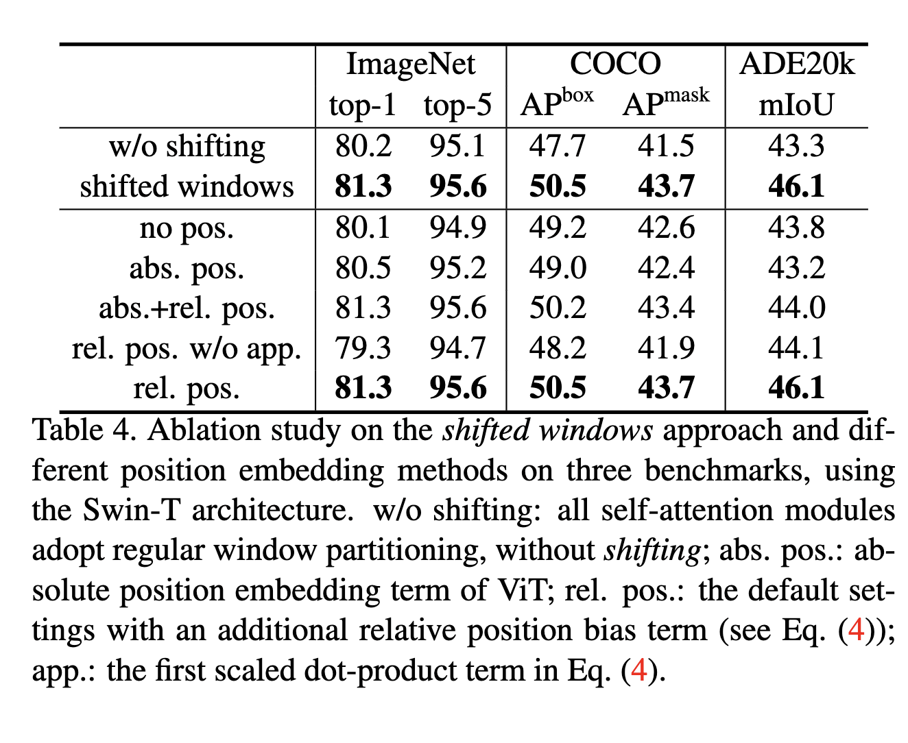
Shifted windows
Ablations of the shifted window approach on the three tasks are reported in Table 4.
세 작업에서 shifted window 접근법의 ablation 결과는 Table 4에 제시되어 있다.
Swin-T with the shifted window partitioning outperforms the counterpart built on a single window partitioning at each stage by +1.1% top-1 accuracy on ImageNet-1K, +2.8 box AP/+2.2 mask AP on COCO, and +2.8 mIoU on ADE20K.
shifted window partitioning을 사용한 Swin-T는
단일 window partition만 사용하는 구조 대비 다음과 같은 성능 향상을 보인다:
- ImageNet-1K: +1.1% top-1 accuracy
- COCO: +2.8 box AP / +2.2 mask AP
- ADE20K: +2.8 mIoU
The results indicate the effectiveness of using shifted windows to build connections among windows in the preceding layers.
이 결과는 shifted window가 이전 레이어의 윈도 간 연결을 형성하는 데 매우 효과적임을 보여준다.
The latency overhead by shifted window is also small, as shown in Table 5.
또한 Table 5에 나타난 것처럼 shifted window 사용による 지연(latency) 증가도 매우 적다.
Relative position bias
Table 4 shows comparisons of different position embedding approaches.
Table 4는 다양한 위치 임베딩 방식의 비교를 보여준다.
Swin-T with relative position bias yields +1.2%/+0.8% top-1 accuracy on ImageNet-1K, +1.3/+1.5 box AP and +1.1/+1.3 mask AP on COCO, and +2.3/+2.9 mIoU on ADE20K in relation to those without position encoding and with absolute position embedding, respectively, indicating the effectiveness of the relative position bias.
relative position bias를 사용한 Swin-T는
위치 인코딩 없음 / absolute position embedding 대비 각각 다음과 같은 향상을 보인다:
- ImageNet-1K: +1.2% / +0.8% top-1 accuracy
- COCO: +1.3 / +1.5 box AP, +1.1 / +1.3 mask AP
- ADE20K: +2.3 / +2.9 mIoU
이는 relative position bias가 매우 효과적임을 보여준다.
Also note that while the inclusion of absolute position embedding improves image classification accuracy (+0.4%), it harms object detection and semantic segmentation (-0.2 box/mask AP on COCO and -0.6 mIoU on ADE20K).
absolute position embedding을 추가하면 이미지 분류에서는 +0.4% 성능이 오르지만,
객체 탐지와 세그멘테이션에서는 오히려 성능이 떨어진다:
- COCO: 0.2 box/mask AP
- ADE20K: 0.6 mIoU
Translation invariance & inductive bias
While the recent ViT/DeiT models abandon translation invariance in image classification even though it has long been shown to be crucial for visual modeling,
최근 ViT/DeiT 모델들은 오랜 기간 시각 모델링에서 핵심으로 여겨졌던 translation invariance(평행 이동 불변성)를 이미지 분류에서 제거했지만,
we find that inductive bias that encourages certain translation invariance is still preferable for general-purpose visual modeling, particularly for the dense prediction tasks of object detection and semantic segmentation.
우리는 translation invariance를 유지하는 inductive bias가 범용 시각 모델링에서 여전히 유리하며,
특히 객체 탐지와 시맨틱 세그멘테이션 같이 dense prediction 작업에서 더 효과적임을 확인했다.
Different self-attention methods
The real speed of different self-attention computation methods and implementations are compared in Table 5.
Table 5에서는 서로 다른 self-attention 계산 방식과 구현 방식의 실제 속도를 비교한다.
Our cyclic implementation is more hardware efficient than naive padding, particularly for deeper stages.
우리의 cyclic-shift 기반 구현은 naive padding 방식보다 하드웨어 효율이 높으며, 특히 네트워크의 깊은 스테이지에서 그 차이가 더 크다.
Overall, it brings a 13%, 18% and 18% speed-up on Swin-T, Swin-S and Swin-B, respectively.
전체적으로 cyclic 구현은 Swin-T, Swin-S, Swin-B에서 각각 13%, 18%, 18%의 속도 향상을 가져온다.
Shifted window vs Sliding window
The self-attention modules built on the proposed shifted window approach are 40.8×/2.5×, 20.2×/2.5×, 9.3×/2.1×, and 7.6×/1.8× more efficient than those of sliding windows in naive/kernel implementations on four network stages, respectively.
shifted window 기반 self-attention 모듈은 슬라이딩 윈도우 방식에 비해
4개 스테이지에서 각각 다음과 같은 효율성을 보인다:
- Stage 1: 40.8× (naive 대비) / 2.5× (kernel 대비)
- Stage 2: 20.2× / 2.5×
- Stage 3: 9.3× / 2.1×
- Stage 4: 7.6× / 1.8×
즉, shifted window 방식은 슬라이딩 윈도우보다 월등히 효율적이다.
Overall, the Swin Transformer architectures built on shifted windows are 4.1/1.5, 4.0/1.5, 3.6/1.5 times faster than variants built on sliding windows for Swin-T, Swin-S, and Swin-B, respectively.
전체적으로 shifted window 기반 Swin Transformer는 슬라이딩 윈도우 기반 변형 모델보다 다음과 같이 빠르다:
- Swin-T: 4.1× (naive 대비) / 1.5× (kernel 대비)
- Swin-S: 4.0× / 1.5×
- Swin-B: 3.6× / 1.5×
즉, 모든 모델에서 sliding window 대비 큰 속도 이점을 가진다.
Table 6 compares their accuracy on the three tasks, showing that they are similarly accurate in visual modeling.
Table 6은 세 작업에서의 정확도를 비교한 것으로, shifted window와 sliding window는 모델링 정확도는 거의 동일함을 보여준다.
Comparison to Performer
Compared to Performer [14], which is one of the fastest Transformer architectures (see [60]),
가장 빠른 Transformer 아키텍처 중 하나인 Performer [14]와 비교했을 때,
the proposed shifted window based self-attention computation and the overall Swin Transformer architectures are slightly faster (see Table 5),
shifted window 기반 self-attention 및 전체 Swin Transformer 구조는 Performer보다 약간 더 빠르며 (Table 5 참조)
while achieving +2.3% top-1 accuracy compared to Performer on ImageNet-1K using Swin-T (see Table 6).
ImageNet-1K에서 Swin-T는 Performer보다 +2.3% top-1 accuracy 더 높은 성능을 보인다(Table 6).
5. Conclusion
This paper presents Swin Transformer, a new vision Transformer which produces a hierarchical feature representation and has linear computational complexity with respect to input image size.
본 논문에서는 입력 이미지 크기에 대해 선형 복잡도를 가지며, 계층적(feature hierarchical) 표현을 생성하는 새로운 비전 Transformer인 Swin Transformer를 제안했다.
Swin Transformer achieves the state-of-the-art performance on COCO object detection and ADE20K semantic segmentation, significantly surpassing previous best methods.
Swin Transformer는 COCO 객체 탐지와 ADE20K 시맨틱 세그멘테이션에서 기존 최고 성능을 크게 넘어서며 최첨단(SOTA) 성능을 달성했다.
We hope that Swin Transformer’s strong performance on various vision problems will encourage unified modeling of vision and language signals.
우리는 Swin Transformer의 다양한 비전 문제에서의 강력한 성능이 비전과 언어 신호의 통합 모델링을 촉진하길 기대한다.
As a key element of Swin Transformer, the shifted window based self-attention is shown to be effective and efficient on vision problems, and we look forward to investigating its use in natural language processing as well.
Swin Transformer의 핵심 요소인 shifted window 기반 self-attention은 비전 문제에서 효과적이고 효율적임이 확인되었으며, 향후 이를 자연어 처리(NLP)에도 적용하는 연구를 기대한다.
Acknowledgement
We thank many colleagues at Microsoft for their help, in particular, Li Dong and Furu Wei for useful discussions; Bin Xiao, Lu Yuan and Lei Zhang for help on datasets.
도움과 지원을 아끼지 않은 Microsoft의 여러 동료들에게 감사드린다. 특히 유익한 논의를 제공한 Li Dong과 Furu Wei, 그리고 데이터셋 관련 도움을 준 Bin Xiao, Lu Yuan, Lei Zhang에게 깊이 감사한다.
A1. Detailed Architectures
The detailed architecture specifications are shown in Table 7, where an input image size of 224×224 is assumed for all architectures.
구체적인 아키텍처 사양은 Table 7에 제시되어 있으며, 모든 아키텍처는 224×224 입력 이미지 크기를 가정한다.
“Concat n × n” indicates a concatenation of n × n neighboring features in a patch.
“Concat n × n”은 패치 내에서 n × n 인접 feature들을 연결(concatenate)하는 연산을 의미한다.
This operation results in a downsampling of the feature map by a rate of n.
이 연산은 feature map을 n배 다운샘플링하는 효과를 가져온다.
“96-d” denotes a linear layer with an output dimension of 96.
“96-d”는 출력 차원이 96인 선형 레이어(linear layer)를 의미한다.
“win. sz. 7 × 7” indicates a multi-head self-attention module with window size of 7 × 7.
“win. sz. 7 × 7”은 윈도 크기 7×7을 사용하는 multi-head self-attention 모듈을 의미한다.
A2. Detailed Experimental Settings
A2.1. Image classification on ImageNet-1K
The image classification is performed by applying a global average pooling layer on the output feature map of the last stage, followed by a linear classifier.
이미지 분류는 마지막 스테이지의 출력 특징 맵에 글로벌 평균 풀링 레이어를 적용한 뒤, 선형 분류기를 이어 붙임으로써 수행된다.
We find this strategy to be as accurate as using an additional class token as in ViT [20] and DeiT [63].
우리는 이 전략이 ViT [20]와 DeiT [63]에서처럼 추가적인 class token을 사용하는 것과 동일한 정확도를 보인다는 것을 확인하였다.
In evaluation, the top-1 accuracy using a single crop is reported.
평가에서는 단일 크롭(single crop)을 사용한 top-1 정확도를 보고한다.
Regular ImageNet-1K training
The training settings mostly follow [63].
훈련 설정은 대부분 [63]을 따른다.
For all model variants, we adopt a default input image resolution of 224².
모든 모델 변형에 대해 기본 입력 이미지 해상도를 224²로 사용한다.
For other resolutions such as 384², we fine-tune the models trained at 224² resolution, instead of training from scratch, to reduce GPU consumption.
384²와 같은 다른 해상도의 경우, GPU 사용량을 줄이기 위해 처음부터 학습하지 않고 224² 해상도에서 학습된 모델을 파인튜닝한다.
When training from scratch with a 224² input, we employ an AdamW [37] optimizer for 300 epochs using a cosine decay learning rate scheduler with 20 epochs of linear warm-up.
224² 입력으로 처음부터 학습할 때는, 20 epoch의 linear warm-up과 함께 cosine decay 학습률 스케줄러를 사용하여 300 epoch 동안 AdamW [37] 옵티마이저를 적용한다.
A batch size of 1024, an initial learning rate of 0.001, a weight decay of 0.05, and gradient clipping with a max norm of 1 are used.
배치 크기 1024, 초기 학습률 0.001, weight decay 0.05, 그리고 최대 노름 1의 gradient clipping을 사용한다.
We include most of the augmentation and regularization strategies of [63] in training, including RandAugment [17], Mixup [77], Cutmix [75], random erasing [82] and stochastic depth [35], but not repeated augmentation [31] and Exponential Moving Average (EMA) [45] which do not enhance performance.
훈련에는 RandAugment [17], Mixup [77], Cutmix [75], random erasing [82], stochastic depth [35]를 포함하여 [63]의 대부분의 증강 및 정규화 전략을 포함하지만, 성능을 향상시키지 않는 repeated augmentation [31]과 지수 이동 평균(EMA) [45]은 사용하지 않는다.
Note that this is contrary to [63] where repeated augmentation is crucial to stabilize the training of ViT.
이는 repeated augmentation이 ViT의 학습을 안정화하는 데 중요했던 [63]과는 반대되는 결과이다.
An increasing degree of stochastic depth augmentation is employed for larger models, i.e. 0.2, 0.3, 0.5 for Swin-T, Swin-S, and Swin-B, respectively.
더 큰 모델일수록 더 높은 비율의 stochastic depth 증강을 사용하며, Swin-T, Swin-S, Swin-B에 대해 각각 0.2, 0.3, 0.5를 사용한다.
For fine-tuning on input with larger resolution, we employ an adamW [37] optimizer for 30 epochs with a constant learning rate of 10⁻⁵, weight decay of 10⁻⁸, and the same data augmentation and regularizations as the first stage except for setting the stochastic depth ratio to 0.1.
더 큰 해상도의 입력으로 파인튜닝할 때는 학습률 10⁻⁵의 고정 학습률, weight decay 10⁻⁸, stochastic depth 비율 0.1을 사용하며, 첫 번째 단계와 동일한 data augmentation 및 정규화를 사용한 채로 AdamW [37] 옵티마이저로 30 epoch 동안 훈련한다.
ImageNet-22K pre-training
We also pre-train on the larger ImageNet-22K dataset, which contains 14.2 million images and 22K classes.
우리는 또한 1,420만 개의 이미지와 22K 개의 클래스를 포함한 더 큰 ImageNet-22K 데이터셋에서 사전 학습을 수행한다.
The training is done in two stages.
훈련은 두 단계로 이루어진다.
For the first stage with 224² input, we employ an AdamW optimizer for 90 epochs using a linear decay learning rate scheduler with a 5-epoch linear warm-up.
224² 입력을 사용하는 첫 번째 단계에서는 5 epoch의 linear warm-up과 linear decay 학습률 스케줄러를 사용하여 90 epoch 동안 AdamW 옵티마이저로 훈련한다.
A batch size of 4096, an initial learning rate of 0.001, and a weight decay of 0.01 are used.
이때 배치 크기 4096, 초기 학습률 0.001, weight decay 0.01을 사용한다.
In the second stage of ImageNet-1K fine-tuning with 224²/384² input, we train the models for 30 epochs with a batch size of 1024, a constant learning rate of 10⁻⁵, and a weight decay of 10⁻⁸.
224²/384² 입력을 사용하는 두 번째 단계의 ImageNet-1K 파인튜닝에서는 배치 크기 1024, 고정 학습률 10⁻⁵, weight decay 10⁻⁸을 사용하여 30 epoch 동안 모델을 훈련한다.
A2.2. Object detection on COCO
For an ablation study, we consider four typical object detection frameworks: Cascade Mask R-CNN [29, 6], ATSS [79], RepPoints v2 [12], and Sparse RCNN [56] in mmdetection [10].
소거 실험(ablation study)을 위해, 우리는 mmdetection [10]의 Cascade Mask R-CNN [29, 6], ATSS [79], RepPoints v2 [12], Sparse RCNN [56]의 네 가지 대표적인 객체 탐지 프레임워크를 고려한다.
For these four frameworks, we utilize the same settings: multi-scale training [8, 56] (resizing the input such that the shorter side is between 480 and 800 while the longer side is at most 1333), AdamW [44] optimizer (initial learning rate of 0.0001, weight decay of 0.05, and batch size of 16), and 3x schedule (36 epochs with the learning rate decayed by 10× at epochs 27 and 33).
이 네 가지 프레임워크에 대해 우리는 동일한 설정을 사용한다: 다중 스케일 학습 [8, 56] (짧은 변을 480~800 사이로, 긴 변은 최대 1333으로 입력을 리사이징), AdamW [44] 옵티마이저 (초기 학습률 0.0001, weight decay 0.05, 배치 크기 16), 그리고 3x 스케줄 (27, 33 epoch에서 학습률을 10배 감소시키는 36 epoch).
For system-level comparison, we adopt an improved HTC [9] (denoted as HTC++) with instaboost [22], stronger multi-scale training [7] (resizing the input such that the shorter side is between 400 and 1400 while the longer side is at most 1600), 6x schedule (72 epochs with the learning rate decayed at epochs 63 and 69 by a factor of 0.1), soft-NMS [5], and an extra global self-attention layer appended at the output of last stage and ImageNet-22K pre-trained model as initialization.
시스템 수준 비교를 위해, 우리는 instaboost [22]가 적용된 향상된 HTC [9] (HTC++로 표기), 더 강력한 다중 스케일 학습 [7] (입력의 짧은 변을 400~1400 사이, 긴 변은 최대 1600으로 리사이징), 6x 스케줄 (63, 69 epoch에서 학습률을 0.1배로 감소시키는 72 epoch), soft-NMS [5], 마지막 스테이지 출력에 추가된 global self-attention 레이어, 그리고 ImageNet-22K 사전학습 모델을 초기값으로 사용한다.
We adopt stochastic depth with ratio of 0.2 for all Swin Transformer models.
모든 Swin Transformer 모델에 대해 stochastic depth 비율 0.2를 적용한다.
A2.3. Semantic segmentation on ADE20K
ADE20K [83] is a widely-used semantic segmentation dataset, covering a broad range of 150 semantic categories.
ADE20K [83]는 널리 사용되는 시맨틱 세그멘테이션 데이터셋으로, 150개의 광범위한 시맨틱 카테고리를 포함한다.
It has 25K images in total, with 20K for training, 2K for validation, and another 3K for testing.
총 25K 이미지로 구성되며, 20K는 훈련용, 2K는 검증용, 그리고 추가 3K는 테스트용이다.
We utilize UperNet [69] in mmsegmentation [16] as our base framework for its high efficiency.
높은 효율성 때문에 우리는 mmsegmentation [16]의 UperNet [69]을 기본 프레임워크로 사용한다.
In training, we employ the AdamW [44] optimizer with an initial learning rate of 6 × 10⁻⁵, a weight decay of 0.01, a scheduler that uses linear learning rate decay, and a linear warmup of 1,500 iterations.
훈련에서는 초기 학습률 6 × 10⁻⁵, weight decay 0.01, 선형 학습률 감소 스케줄러, 그리고 1,500 iteration의 linear warmup을 사용하는 AdamW [44] 옵티마이저를 적용한다.
Models are trained on 8 GPUs with 2 images per GPU for 160K iterations.
모델은 GPU당 2개의 이미지를 사용하여 총 8개의 GPU에서 160K iteration 동안 훈련된다.
For augmentations, we adopt the default setting in mmsegmentation of random horizontal flipping, random re-scaling within ratio range [0.5, 2.0] and random photometric distortion.
증강으로는 mmsegmentation의 기본 설정인 랜덤 수평 뒤집기, 비율 범위 [0.5, 2.0] 내 랜덤 리스케일링, 랜덤 photometric distortion을 사용한다.
Stochastic depth with ratio of 0.2 is applied for all Swin Transformer models.
모든 Swin Transformer 모델에 stochastic depth 비율 0.2가 적용된다.
Swin-T, Swin-S are trained on the standard setting as the previous approaches with an input of 512×512.
Swin-T, Swin-S는 이전 접근 방식과 동일한 표준 설정에서 512×512 입력으로 훈련된다.
Swin-B and Swin-L with ‡ indicate that these two models are pre-trained on ImageNet-22K, and trained with the input of 640×640.
‡ 표시가 있는 Swin-B와 Swin-L은 ImageNet-22K에서 사전 학습된 모델이며 640×640 입력으로 훈련된다.
In inference, a multi-scale test using resolutions that are [0.5, 0.75, 1.0, 1.25, 1.5, 1.75]× of that in training is employed.
추론에서는 훈련 시 입력 해상도의 [0.5, 0.75, 1.0, 1.25, 1.5, 1.75]배 스케일을 사용하는 다중 스케일 테스트가 적용된다.
When reporting test scores, both the training images and validation images are used for training, following common practice [71].
테스트 점수를 보고할 때는 일반적인 관례 [71]에 따라 훈련 이미지와 검증 이미지를 모두 훈련에 사용한다.
A3. More Experiments
A3.1. Image classification with different input size
Table 8 lists the performance of Swin Transformers with different input image sizes from 224² to 384².
표 8은 224²부터 384²까지의 서로 다른 입력 이미지 크기에 따른 Swin Transformer의 성능을 나열한다.
In general, a larger input resolution leads to better top-1 accuracy but with slower inference speed.
일반적으로 더 큰 입력 해상도는 더 나은 top-1 정확도를 제공하지만 추론 속도는 더 느려지게 된다.
A3.2. Different Optimizers for ResNe(X)t on COCO
Table 9 compares the AdamW and SGD optimizers of the ResNe(X)t backbones on COCO object detection.
표 9는 COCO 객체 탐지에서 ResNe(X)t 백본에 대해 AdamW 옵티마이저와 SGD 옵티마이저를 비교한다.
The Cascade Mask R-CNN framework is used in this comparison.
이 비교에서는 Cascade Mask R-CNN 프레임워크가 사용된다.
While SGD is used as a default optimizer for Cascade Mask R-CNN framework, we generally observe improved accuracy by replacing it with an AdamW optimizer, particularly for smaller backbones.
Cascade Mask R-CNN 프레임워크는 기본적으로 SGD를 옵티마이저로 사용하지만, AdamW 옵티마이저로 교체할 경우 일반적으로 더 나은 정확도가 관찰되며, 특히 더 작은 백본에서 두드러진다.
We thus use AdamW for ResNe(X)t backbones when compared to the proposed Swin Transformer architectures.
따라서 제안된 Swin Transformer 아키텍처와 비교할 때 ResNe(X)t 백본에는 AdamW를 사용한다.
A3.3. Swin MLP-Mixer
We apply the proposed hierarchical design and the shifted window approach to the MLP-Mixer architectures [61], referred to as Swin-Mixer.
우리는 제안된 계층적 설계와 shift된 윈도우 접근 방식을 MLP-Mixer 아키텍처 [61]에 적용하며, 이를 Swin-Mixer라고 부른다.
Table 10 shows the performance of Swin-Mixer compared to the original MLP-Mixer architectures MLP-Mixer [61] and a follow-up approach, ResMLP [62].
표 10은 Swin-Mixer의 성능을 원본 MLP-Mixer 아키텍처인 MLP-Mixer [61] 및 후속 접근 방식인 ResMLP [62]와 비교하여 보여준다.
Swin-Mixer performs significantly better than MLP-Mixer (81.3% vs. 76.4%) using slightly smaller computation budget (10.4G vs. 12.7G).
Swin-Mixer는 약간 더 작은 연산 예산(10.4G vs. 12.7G)을 사용하면서도 MLP-Mixer보다 현저히 더 높은 성능(81.3% vs. 76.4%)을 보인다.
It also has better speed-accuracy trade-off compared to ResMLP [62].
또한 ResMLP [62]와 비교해도 더 나은 속도–정확도 균형을 보여준다.
These results indicate the proposed hierarchical design and the shifted window approach are generalizable.
이러한 결과는 제안된 계층적 설계와 shift된 윈도우 접근 방식이 일반화 가능함을 나타낸다.