Review - Mean Squared Error(MSE)

• Mean Squared Error(MSE) criterion

  $mse(\hat \theta) = E[(\hat \theta -\theta)^2] =var(\hat \theta) + b^2(\theta)$

• Note that, in many cases, minimum MSE criterion leads to unrealizable estimator, which cannot be written solely as a function of the data, i.e.,

  $\widecheck A =a\dfrac{1}{N}\displaystyle\sum_{n=0}^{N-1}x[n],\;A\;:\;unknown\\objective\;:\;estimate\;A\;from\;x[n]$

  • where $\textcolor{red}{\alpha}$ is choosen to minimize MSE

    $E(\widecheck A)=\textcolor{red}\alpha A,\;var(\widecheck A)=\dfrac{a^2\sigma^2}{N} \rightarrow mse(\widecheck A)=\dfrac{a^2\sigma^2}{N}+(a-1)^2A^2\\[0.4cm] \therefore a_{opt}=\dfrac{A^2}{A^2+\sigma^2/N}$

    $$

Review - MVUE

• Minimum variance unbiased estimator(MVUE)
• Alternatively, constrain the bias to be zero
• Find the estimator which minimizes the variance $\cdots\textcolor{red}{~ (*)}$
  • Minimuzing the MSE as well for unbiased case

    $mse(\hat \theta)=var(\hat \theta) +b^2(\theta)=var(\hat \theta),\;E[b^2(\theta)]=0 \;\cdots\textcolor{red}{~ (*)}$

• That's Minimum variance unbiased estimator so called MVUE
  
• Then... how can we know MVUE Exsist!!!?

Outline

• Cramer-Rao Lower Bound(CRLB)
• Estimator Accuracy Considerations
• CRLB for a Scalar Parameter
• CRLB Proof
• General CRLB for Signals in WGN
• Transformation of Parameters
• Vector form of the CRLB
• General Gaussian Case and Fisher Infromation

Cramer-Rao Lower Bound(CRLB)

• Cramer-Rao Lower Bound(CRLB) or Cramer-Rao Bound(CRB) - Same things
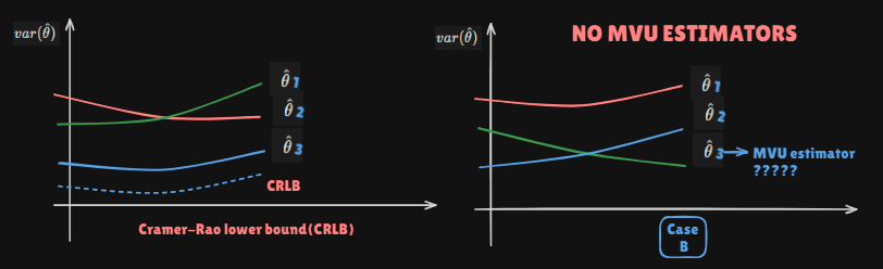
• The CRLB give a lower bound on the variance of any unbiased estimator

  Does not guarantee bound can be obtained

• If one finds out an unbiased estimator whose variance = CRLB then it's MVUE(very very very very ideal cases...)
• Otherwise can use Ch.5 tools(Rao-Blackwell-Lehmann-Scheffe Teorem and Neyman-Fisher Facorization Theorem) to construct a better estimator from any unbiased one-possibly the MVUE if condidtions are met

Estimator Accuracy Considerations

• All information is observed data and underlying PDF
  • Estimation accuracy depends directly on the PDF
• For example) PDF dependence on unknown parameter

  Signal sample observation

  $x[0]=A+w[0],\;w[0] \sim \mathcal{N}(0, \sigma^2)\\ \mathcal{N}(0, \sigma^2)\;:\;Adaptive\;White\;Gaussian\;Noise$

  • Good unbiased estimator : $\hat A =x[0]$
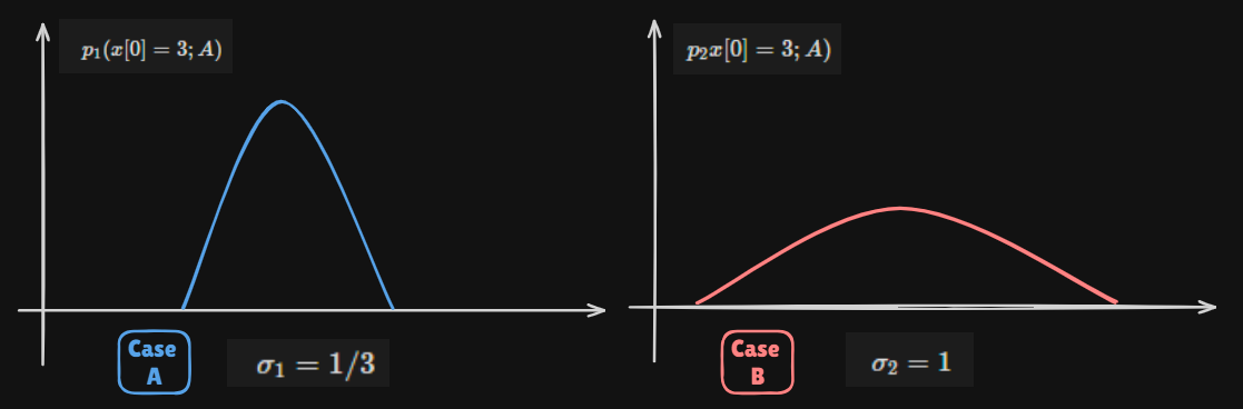
  • The smaller $\sigma^2$ is, the better the estimator accuracy is
  • Alternatively, likelihood function($\neq$PDF)

    $p_i(x[0];A)=\dfrac{1}{\sqrt{2\pi\sigma_i^2}}exp\left[-\dfrac{1}{2\sigma_i^2}(x[0]-A)^2\right]$

    

• Likelihood : What is Prob for $\theta =A$, Variance indicates how estimators Accurate
• The Sharpness of the likelihood function determines the accuracy of the estimate
• Measured by the curvature of the log-likelihood function
  • It's negative of the second derivative of the logarithm of the likelihood function at its peak. i.e.,

    $lnp(x[0];A)=-ln\sqrt{2\pi\sigma^2}-\dfrac{1}{2\sigma^2}(x[0]-A^2),\\ \dfrac{\partial^2}{\partial A^2} \rightarrow -ln\sqrt{2\pi\sigma^2}=0,\;no\;A\;dependency\\[0.5cm] -\dfrac{\partial^2 lnp(x[0];A)}{\partial A^2}=\dfrac{1}{\sigma^2},\quad var(\hat A)=\sigma^2=\dfrac{1}{\dfrac{\partial^2lnp(x[0];A)}{\partial A^2}}$

  • Average curvature : $-E\left[\dfrac{\partial ^2ln\;p(x[0];A}{\partial A^2}\right]$
    • In general, the $2^{nd}$ derivative will depend on $x[0] \rightarrow$ the likelihood function is a R.V.

Theorem : Cramer-Rao Lower Bound(CRLB) - Scalar Parameter

• Let $p(x;\theta)$ satify the regularity condition :

  $E\left[\dfrac{\partial \;ln\;p(x;\theta)}{\partial \theta}\right]=0\;for\;all\;\theta$

• Then, the variance of any unbiased estimator $\hat \theta$ must satisfy

  $var(\hat \theta)\geq\dfrac{1}{-E\left[\dfrac{\partial^2\;ln\;p(x;\theta)}{\partial \theta^2}\right]}=\dfrac{1}{E\left[\left(\dfrac{\partial\;ln\;p(x;\theta)}{\partial\theta}\right)^2\right]}$

• Where the derivative is evaluated at the true value of $\theta$ and the expectation is taken w.r.t. $p(x;\theta)$
• Furthermore, an unbiased estimator may be founc that attains the bound for all $\theta$ if and only if

  $\dfrac{\partial\;ln\;p(x;\theta)}{\partial \theta}=I(\theta)(g(x)-\theta)$

• For some functions $g(x)$ and $I$. That estimator, which is the MVUE, is $\hat \theta =g(x)$, and the`minimum variance is $1/I(\theta)$

  To sum up : If some functions's logarithm cavarture could be decomposed just like $I(\theta)(g(x)-\theta)$
  Then $g(x)$ is MVUE

CRLB Proof (Appendix 3A)

• CRLB for a scalar parameter $\alpha =g(\theta)$ where the PDF is parameterized with $\theta$.

• Consider unbiased estimator $\hat \alpha$, i.e.,

  $E(\hat \alpha) =\int\hat ap(x;\theta)dx=\alpha=g(\theta)\cdots\textcolor{red}{(*)}$

• Regularity condition : holds if the order of differentiation and integration may be interchanged

  $E\left[\dfrac{\partial\;ln\;p(x;\theta)}{\partial \theta}\right]=\int\dfrac{\partial\;ln\;p(x;\theta)}{\partial\theta}p(x;\theta)dx=0$

• Differentiating both sides of $\textcolor{red}{(*)}$

  $\int\hat \alpha\dfrac{\partial\;p(x;\theta)}{\partial\theta}dx=\dfrac{\partial\;g(\theta)}{\partial \theta}\\ \rightarrow \int\hat \alpha\dfrac{\partial\;ln\;p(x;\theta)}{\partial \theta}p(x;\theta)dx\cdots\textcolor{red}{(**)}=\dfrac{\partial g(\theta)}{\partial \theta}$

  $\dfrac{\partial}{\partial\theta}ln\;C(\theta)=\dfrac{1}{C(\theta)}\dfrac{\partial\;C(\theta)}{\partial\theta},\;C(\theta)=P(x;\theta)\cdots\textcolor{red}{(**)}$

• By using regularity condition,

  $\int\textcolor{blue}{(\hat \alpha-\alpha)}\dfrac{\partial \;ln\;p(x;\theta)}{\partial \theta}p(x;\theta)dx=\dfrac{\partial\;g(\theta)}{\partial\theta}$

• By using Cauchy-Schwarz inequality,

  $\left(\dfrac{\partial g(\theta)}{\partial\theta}\right)^2\leq\int(\hat \alpha -\alpha)^2p(x;\theta)dx\int\left(\dfrac{\partial\;ln\;p(x;\theta)}{\partial\theta}\right)^2p(x;\theta)dx\\[0.5cm] \int(\hat\alpha-\alpha)^2p(x;\theta)dx=E[(\hat \alpha-E[\hat \alpha])^2=E[(\hat \alpha-\alpha)^2]\\[0.5cm] \therefore var(\hat \alpha) \geq \dfrac{\left(\dfrac{\partial\;g(\theta)}{\partial\theta}\right)^2}{E\left[\left(\dfrac{\partial\;ln\;p(x;\theta)}{\partial \theta}\right)^2\right]}$

  Cauchy-Schwarz Inequality

  $\left[\int w(x)g(x)h(x)dx\right]^2\leq\int w(x)g^2(x)dx\int w(x)h^2(x)dx$

  • Arbitrary function $g(x)$ and $h(x)$, while $w(x)\geq0$ for all $x$.
  • Equality holds in and only if
    $g(x)=c\;h(x)$

• By differentiating the regularity condition,

  $\dfrac{\partial}{\partial\theta}\int\dfrac{\partial\;ln\;p(x;\theta)}{\partial\theta}p(x;\theta)dx=0\\[0.5cm] \int\left[\dfrac{\partial^2\;ln\;p(x;\theta)}{\partial\theta^2}p(x;\theta)+\dfrac{\partial\;ln\;p(x;\theta)}{\partial\theta}\dfrac{\partial p(x;\theta)}{\partial\theta}\right]dx=0\\[0.5cm] -E\left[\dfrac{\partial^2\;ln\;p(x;\theta)}{\partial \theta^2}\right]=\int \dfrac{\partial\;ln\;p(x;\theta)}{\partial\theta}\dfrac{\partial\;ln\;p(x;\theta)}{\partial\theta}p(x;\theta)dx\\[0.5cm] =E\left[\left(\dfrac{\partial\;ln\;p(x;\theta)}{\partial \theta}\right)^2\right]\\[0.5cm] \rightarrow var(\hat \alpha)\geq\dfrac{\left(\dfrac{\partial\;g(\theta)}{\partial\theta}\right)^2}{E\left[\left(\dfrac{\partial\;ln\;p(x;\theta)}{\partial\theta}\right)^2\right]}=\dfrac{\left(\dfrac{\partial\;g(\theta)}{\partial\theta}\right)^2}{-E\left[\dfrac{\partial^2\;ln\;p(x;\theta)}{\partial\theta^2}\right]}$

• $\text{if} \;\alpha=g(\theta)=\theta,$
  $\text{var}(\hat{\theta}) \geq \frac{1}{-E \left[ \frac{\partial^2 \ln p(x; \theta)}{\partial \theta^2} \right]} = \frac{1}{E \left[ \left( \frac{\partial \ln p(x; \theta)}{\partial \theta} \right)^2 \right]}\\ \text{Condition for equality:}\\ \frac{\partial lnp(x;\theta)}{\partial\theta}=\frac{1}{c}(\hat \alpha-\alpha),\;\hat \alpha=\text{MVUE}\\ \frac{\partial ln p(x;\theta)}{\partial \theta}=\frac{1}{c(\theta)}(\hat \theta - \theta)\\ \text{To determine c(}\theta\text{)},\\ \frac{\partial^2 ln p(x;\theta)}{\partial\theta^2}=-\frac{1}{c(\theta)}+\frac{\partial(\frac{1}{c(\theta)})}{\partial\theta}(\hat \theta - \theta)\\[0.3cm] -E[\frac{\partial^2 ln p(x;\theta)}{\partial \theta^2}=\frac{1}{c(\theta)}=I(\theta)$

CRLB Example - DC Level in WGN

Let $\hat A = \hat x$, then it is MVUE

CRLB Example - Phase Estimation

for $f_0$ not near 0 or $\frac{1}{2}$
$\rightarrow\text{var}(\hat\phi)\geq\frac{2\sigma^2}{NA^2}$
but the condition for bound to hold is not satisfied. MVUE may exist and indded can be found with sufficient statistics(Chap. 5)

Efficient Estimator and Fisher Information

• Efficient estimator
  • An unbiased estimator that attains the CRLB
  • MVUE may or may not be efficient

    Fisher Information
    $I(\theta)=-E\left[\frac{\partial^2 ln p(x;\theta)}{\partial \theta^2}\right]=E\left[\left(\frac{\partial ln p (x;\theta)}{\partial \theta}\right)^2\right]$

  • Why "Information"?
    • The more information, the lower the bound
    • Non-negative
    • Additive for independent observations

  CRLB True or False

• The CRLB always exists regardless of $p(x;\theta)$ : False, regularity condition
• The CRLB applies to unbiased estimators only : True
• Determining the CRLB requires statistics of all possible estimators $\hat \theta$ : False, likelihood $P(\bar x;\theta)$
• The CRLB depends on the observations $x$ : False, applied expectations, removing dependency
• The CRLB depends on the parameter to be estimated $\theta$ : True
• The CRLB tells you whether or not a MVUE exists False, don't tell anything about MVUE

General CRLB for Signals in WGN

Transformation of Parameters

Wish to estimate $\alpha = g(\theta)$ instead of $\theta$ itself,

Ex) DC level in WGN, $\alpha =g(A) =A^2$(non-linear transformation)

• Is $\bar x^2$ efficient for $A^2$?
  • if variance of $\bar x^2$ hitting bound : it's efficient
  • variance is now function of $A$
    • We know the Bound
    • We don't know how to find it

Linear transformation: $g(\theta) =a\theta +b$

Since $var(\hat{g(\theta)}=a^2\text{var}(\hat\theta)$ : CRLB is achieved

• Else if, Efficiency is approximately maintained over nonlinear transformations if the data record is large enough.
  Ex) DC level in WGN, estimate $A^2$ with $\hat{A^2}=\bar x^2, \text{var}(\hat A^2)\geq\frac{(2A)^2}{\frac{N}{\sigma^2}}=\frac{4A^2\sigma^2}{N}$

Statiscal linearity of the trasformation : linear approximation is possible when the PDF of the $\bar x$ is concentrated about the mean $A$.
Even though Non-Linear : We can get CRLB

Vector Form of the CRLB

When the parameter $\theta = [\theta_1\;\theta_2\;\cdots\;\theta_p]^T$, we now have a bound on the entire covariance matrix $C_{\hat\theta}$ of any estimator $\hat\theta$ of $\theta$.
The Fisher Information Matrix is the quantity of importance here, and is the generalization of $I(\theta)$ to the vector case. It is a $p\times p$ matrix of second partials of the log likelihood function. Fisher Information Matrix's $i,\;j$ entry is

where expectations are again taken over $p(x;\theta)$.

• Assuming $p(x;\theta)$ satisfies the regularity condition
  $E\left[\frac{\partial ln p(x;\theta)}{\partial\theta}\right]=0,\quad \text{for all }\theta$
• The covariance matrix of any unbiased estimator $\hat \theta$ satisfies
  $C_{\hat \theta}-I^{-1}(\theta) \geq 0$
  where $\geq 0$ means the matrix is positive semidefinite.
• Furthermore, an unbiased estimator may be found that attains the bound $C_{\hat\theta}=I^{-1}(\theta)$ if and only if
  $\frac{\partial ln p(x;\theta)}{\partial\theta}=I(\theta)(g(x)-\theta)$

  In that case, $\hat \theta =g(x)$ is the MVU estimator with variance $I^{-1}(\theta)$

Vector Form of the CRLB - Example

Ex) DC level in AWGN with unkwnown noise variance : $\theta = [A \; \sigma^2]^T$ (estimating the vector of parameters)

• The Fisher information matrix would be,
  $I(\theta) = \begin{bmatrix} -E\left[ \frac{\partial^2 \ln p(x; \theta)}{\partial A^2} \right] & -E\left[ \frac{\partial^2 \ln p(x; \theta)}{\partial A \partial \sigma^2} \right] \\ -E\left[ \frac{\partial^2 \ln p(x; \theta)}{\partial A \partial \sigma^2} \right] & -E\left[ \frac{\partial^2 \ln p(x; \theta)}{\partial \sigma^4} \right] \end{bmatrix}\\ \ln p(x; \theta) = -\frac{N}{2} \ln 2\pi - \frac{N}{2} \ln \sigma^2 - \frac{1}{2\sigma^2} \sum_{n=0}^{N-1} (x[n] - A)^2\\ \frac{\partial \ln p(x; \theta)}{\partial A} = \frac{1}{\sigma^2} \sum_{n=0}^{N-1} (x[n] - A)\\ \frac{\partial \ln p(x; \theta)}{\partial \sigma^2} = -\frac{N}{2\sigma^2} + \frac{1}{2\sigma^4} \sum_{n=0}^{N-1} (x[n] - A)^2\\ \frac{\partial^2\ln p(x;\theta)}{\partial A^2}=-\frac{N}{\sigma^2}\\ \frac{\partial^2 \ln p(x; \theta)}{\partial A \partial \sigma^2} = - \frac{1}{\sigma^4} \sum_{n=0}^{N-1} (x[n] - A)\\ \frac{\partial^2 \ln p(x; \theta)}{\partial \sigma^2} = \frac{N}{2\sigma^4} - \frac{1}{\sigma^6} \sum_{n=0}^{N-1} (x[n] - A)^2\\ \rightarrow I(\theta) = \begin{bmatrix} \frac{N}{\sigma^2} & 0 \\ 0 & \frac{N}{2\sigma^4} \end{bmatrix}$
• Diagonal Fisher information matrix, $var(\hat A) \geq \frac{\sigma^2}{N}, var(\hat \sigma^2 ) \geq \frac{2\sigma^4}{N}$

Vector CRLB for Transformations

• Estimate $\alpha = g(\theta)$ for $g$, an r-dimensional function
• The covariance matrix $C_{\hat \alpha}$ of any unbiased estimator $\hat \alpha$(From Appendix 3B)
  $C_{\hat \alpha}-\frac{\partial g(\theta)}{\partial \theta}I^{-1}(\theta)\frac{\partial g(\theta)^T}{\partial \theta} \geq 0$
• Here, $\partial g(\theta)/\partial\theta$ is the $r\times p$ Jacobian matrix, whose elements are
  $\left[\frac{\partial g(\theta)}{\partial \theta}\right]_{i,j}=\frac{\partial g_j(\theta)}{\partial \theta}$

CRLB for General Gaussian Case

• When observations are Gaussian and one knows the dependence of the mean and covariance matrix on the unknown parameters, we know the closed form of the CRLB(or Fisher information matrix):
  $\mathbf{x} \sim \mathcal{N}(\mu(\theta), C(\theta)),$
• Then, the Fisher information matrix $I(\theta)$ is given by:
  $[I(\theta)]_{i,j}=\left[\frac{\partial \mu(\theta)}{\partial\theta_i}\right]^T C^{-1}(\theta)\left[\frac{\partial \mu(\theta)}{\partial \theta_j}\right] +\frac{1}{2}\text{tr}\left[C^{-1}(\theta)\frac{\partial C(\theta)}{\partial \theta_i} C^{-1} (\theta)\frac{\partial C(\theta)}{\partial \theta_j}\right]$

Phase Estimation CRLB

• Phase estimation example, $x[n]=A\text{cos}(2\pi f_0 n+\phi) +w[n]$
  $\text{var}(\hat\phi)\geq\frac{2\sigma^2}{NA^2}$
• Does an efficient estimator exist for this problem? The CRLB theorem says there is only if
  $\frac{\partial \ln p(x;\theta)}{\partial \theta}=I(\theta)(g(x)-\theta)$
• From earlier result,
  $\frac{\partial \ln p(x; \phi)}{\partial \phi} = - \frac{A}{\sigma^2} \sum_{n=0}^{N-1} \left[ x[n] \sin(2\pi f_0 n + \phi) \right] - \frac{A}{2} \sin(4\pi f_0 n + 2\phi)$
• The condition for bound to hod is not satisfied!
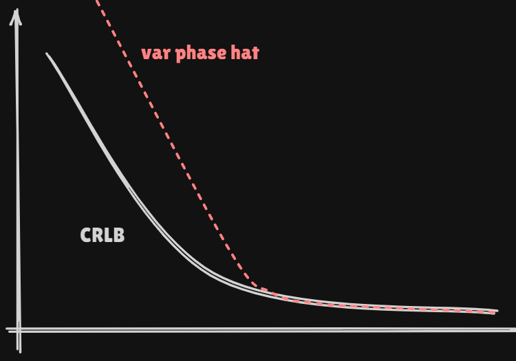
• We saw the estimator for which $\text{var}(\hat\phi) \rightarrow CRLB \;as\; N \rightarrow \infty$
  
• Such an estimator is called an asymptotically efficient estimator

Range Estimation CRLB

• Transmit pulse $s(t)$, nonzero over $t \in [0,T_s]$

• Receive reflection $s(t-\tau_0)$

• Estimation of time delay $\tau_0$, since the round trip delay $\tau_0 =2R/c$

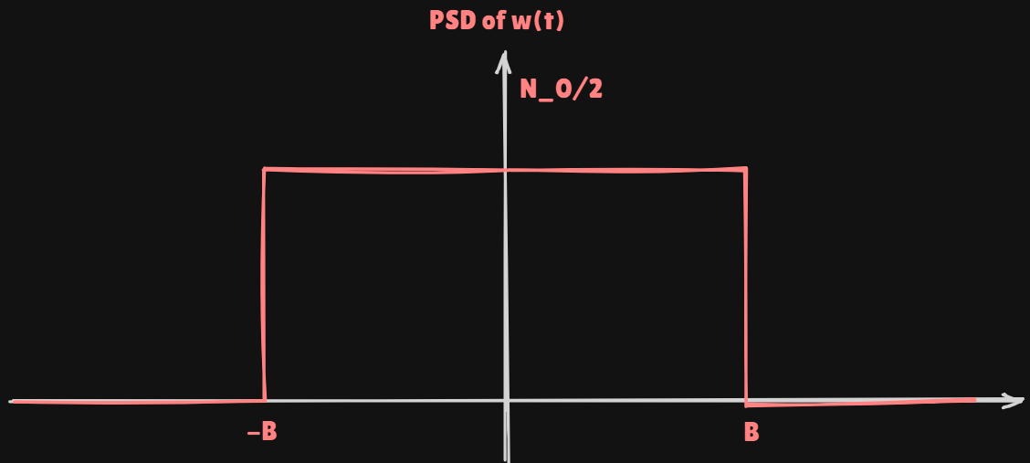
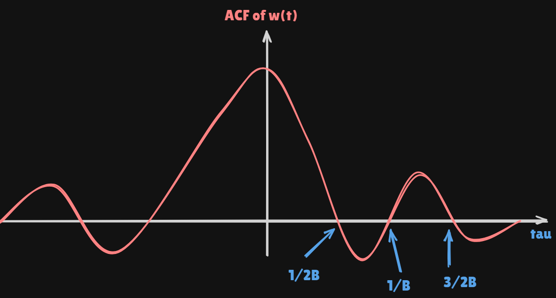
  Continuous time signal model
  $x(t) = s(t-\tau_0)+w(t) \quad 0\leq t\leq T=T_s+\tau_{0max}$
  
  
  $r_{ww}(\tau) = N_0 B \frac{\sin(2\pi \tau B)}{2\pi \tau B}$

• Discrete time signal model

  • Sample every $\delta=1/(2B)$ sec
    $s[n]=s(n\delta-\tau_0)+w[n]\quad n=0,1,\dots,N-1$
  • $s(n\delta-\tau_0)$ has $M$ non-zero samples at $n_0$
    $x[n] = \begin{cases} w[n] & 0 \leq n \leq n_0 - 1 \\ s(n\Delta - \tau_0) + w[n] & n_0 \leq n \leq n_0 + M - 1 \\ w[n] & n_0 + M \leq n \leq N - 1 \end{cases}$

• Now apply standard CRLB result for signal + WGN

  $\text{var}(\hat{\tau_0}) \geq \frac{\sigma^2}{\sum_{n=0}^{N-1} \left( \frac{\partial s[n; \tau_0]}{\partial \tau_0} \right)^2}\\[0.4cm] = \frac{\sigma^2}{\sum_{n=n_0}^{n_0+M-1} \left( \frac{\partial s(n\Delta - \tau_0)}{\partial \tau_0} \right)^2}\\[0.4cm] = \frac{\sigma^2}{\sum_{n=n_0}^{n_0+M-1} \left( \frac{\partial s(t)}{\partial t} \Big|_{t = n\Delta - \tau_0} \right)^2}\\[0.4cm] = \frac{\sigma^2}{\sum_{n=0}^{M-1} \left( \frac{\partial s(t)}{\partial t} \Big|_{t = n\Delta} \right)^2}$

• Assume sample spacing is samll...approx. sum by integral...

  $\text{var}(\hat{\tau_0}) \geq \frac{\sigma^2}{\frac{1}{\Delta} \int_0^{T_s} \left( \frac{\partial s(t)}{\partial t} \right)^2 dt}\\[0.4cm] = \frac{N_0 / 2}{\int_0^{T_s} \left( \frac{\partial s(t)}{\partial t} \right)^2 dt}\\[0.4cm] = \frac{1}{\frac{E_s}{N_0 / 2} \cdot \frac{1}{E_s} \int_0^{T_s} \left( \frac{\partial s(t)}{\partial t} \right)^2 dt}\\[0.4cm] = \frac{1}{\text{SNR} \cdot B_{\text{rms}}^2} \, \text{(sec}^2\text{)}$

• Using these ideas we arrive at the CRLB on the delay:

  $\text{var}(\hat{\tau_0}) \geq \frac{1}{\text{SNR} \cdot B_{\text{rms}}^2} \, \text{(sec}^2\text{)}$

• To get the CRLB on the range use transf. of params result with $R=c\tau_0/2$

  $\text{CRLB}_{\hat{R}} = \left( \frac{\partial R}{\partial \tau_0} \right)^2 \text{CRLB}_{\hat{\tau_0}}\\[0.4cm] \text{var}(\hat{R}) \geq \frac{c^2 / 4}{\text{SNR} \cdot B_{\text{rms}}^2} \, (\text{m}^2)$

• CRLB is inversely proportional to SNR and RMS BW Measure

  All Content has been written based on lecture of Prof. eui-seok.Hwang in GIST(Detection and Estimation)