Review of Finding the MVUE

• When the observation and the data are related in a linear way $\text{x}=\text{H}\theta+\text{w}$
• And the noise was Gaussian, then the MVUE was easy to find :
  $\hat\theta=(\text{H}^T\text{H})^{-1}\text{H}^T\text{x}$
  with covariance matrix, $C_{\hat\theta}=I^{-1}(\theta)=\sigma^2(\text{H}^T\text{H})^{-1}$
• Using the CRLB, if you got lucky, you could write
  $\frac{\partial \ln p(x;\theta)}{\partial \theta}=I(\theta)(g(x)-\theta)$
  where $\hat \theta = g(x)$ would be your MVUE, which would also be an efficient estimator(meeting the CRLB)
• Even if no efficient estimator exists, an MVUE may exist

  A systematic way of determining the MVUE is introduced, if it exists

---

• We wish to estimate the parameter(s) $\theta$ from the observations $\text{x}$
• Step 1
  • Determine (if possible) a sufficient statistic $T(x)$ for the paramter to be estimated $\theta$
  • This may be done using the Neyman-Fisher factorization theorem
• Step 2
  • Determine whether the sufficient statistic is also complete
  • This is generally hard to do
  • If it is not complete, we can say nothing more about the MVUE
  • If it is, continue to Step 3
• Step 3
  • Find the MVUE $\hat\theta$ from $T(x)$ is one of two ways using the Rao-Blackwell-Lehmann-Scheffe(RBLS) theorem :
    • Find a function $g(\cdot)$ of the sufficient statistic that yields an unbiased estimator $\hat\theta = g(T(x))$, the MVUE
    • By definition of completeness of the statistic, this will yield the MVUE
  • Find any unbiased estimator $\check\theta$ for $\theta$
    • And then determine $\hat\theta=E[\check\theta|T(x)]$
    • This is usually very difficult to do
    • The expectation is taken over the distribution $p(\check\theta|T(x))$

---

Motivation for MVUE

• MVUE often does not exist or can't be found!

  Solution : If the PDF is known, then MLE can always be used!!
  (MLE is one of the most popular practical methods)

• Advantages
  • It is a "Turn-The-Crank" method
  • Optimal for large enough data size
• Disadvantages
  • Not optimal for small data size
  • Can be computationally complex, may require numerical methods

CRLB/RBLS Not Applicable Example

• DC Level in WGN w/ unknown variance
  (Either CRLB theorem or RBLS theorem is not applicable)
  $x[n]=A+w[n],\quad n=0,1,\cdots,N-1$
  $A$ : unknown level $(A>0)$, $w[n]$ : WGN with unknown variance $A$
  $p(\text{x};A)=\frac{1}{(2\pi A)^{N/2}}\exp\left[-\frac{1}{2A}\sum_{n=0}^{N-1}(x[n]-A)^2\right]\\[0.3cm]$
• $x[n]\sim\mathcal{N}(A,A)$
• $E[x[n]]=A$
• $E[x^2[n]]=\text{Var}[x[n]]+E^2[x[n]]=A+A^2$

---

• Firstly, check if CRLB theorem can give an efficient estimator :
  $\frac{\partial\ln p(x;A)}{\partial A}=-\frac{N}{2A} + \frac{1}{A}\sum_{n=0}^{N-1} (x[n]-A)+\frac{1}{2A^2}\sum_{n=0}^{N-1}(x[n]-A)^2\\[0.3cm] =-\frac{N}{2A}+\frac{1}{A}\sum_{n=0}^{N-1}x[n]-N+\frac{1}{2A^2}\sum_{n=0}^{N-1}x^2[n]-\frac{1}{A}\sum_{n=0}^{N-1}x[n]+\frac{N}{2}\\[0.3cm] =-\frac{N}{2A}-N+\frac{1}{2A^2}\sum_{n=0}^{N-1}x^2[n]+\frac{N}{2}\\[0.3cm] =-\frac{N}{2A}-\frac{N}{2}+\frac{1}{2A^2}\sum_{n=0}^{N-1}x^2[n]$
  : cannot be factored as $I(A)(g(x)-A)$, so an efficient estimator cannot be founc, but CRLB is given
  $\text{var}(\hat A)\geq\frac{1}{-E\left[\frac{\partial^2\ln p(x;A)}{\partial A^2}\right]}=\frac{A^2}{N(A+\frac{1}{2})}\\[0.3cm[] \frac{\partial^2\ln p(x;A)}{\partial A^2}=\frac{N}{2A^2}-\frac{1}{A^3}\sum_{n=0}^{N-1}x^2[n]\\[0.3cm] -E\left[\frac{\partial^2\ln p(x;A)}{\partial A^2}\right]=-\frac{N}{2A^2}+\frac{1}{A^3}N\cdot (A+A^2)\\[0.3cm] =\frac{1}{A^2}N(A+\frac{1}{2})$

---

• Next, we try to find the MVUE based on sufficient statistics
  $p(\mathbf{x}; A) = \frac{1}{(2\pi A)^{N/2}} \exp \left[ - \frac{1}{2A} \left( \sum_{n=0}^{N-1} x[n]^2 - 2A \sum_{n=0}^{N-1} x[n] + NA^2 \right) \right]\\[0.3cm] = \frac{1}{(2\pi A)^{N/2}} \exp \left[ -\frac{1}{2} \left( \frac{1}{A} \sum_{n=0}^{N-1} x[n]^2 + NA \right) \right] \exp(N \bar{x})$
• $T(x)=\sum_{n=0}^{N-1}x^2[n]$ is a single sufficient statistic for $A$ by Neyman-Fisher factorization theorem
• Assuming that $T(x)$ is complete, find a function $g$ of $T(x)$ that produces an unbiased estimator
  $E\left[\sum_{n=0}^{N-1}x^2[n]\right]=NE[x^2[n]]\\[0.3cm] =N[\text{var}(x[n])+E^2(x[n])]\\ =N(A+A^2)$
• It is not obvious how to choose $g$
• Alternative way is to evaluate $E[\check A|T(x)] =E[x[0]|\sum_{n=0}^{N-1}x^2[n]]$, which is quite challenging

Approximately Optimal Estimator

• Cannot find an MVUE : propose an estimator that is approximately optimal
  $\text{As } N \to \infty, \quad \begin{cases} E(\hat{A}) \to A \quad \text{(asymptotically unbiased)} \\ \text{var}(\hat{A}) \to \text{CRLB} \quad \text{(asymptotically efficient)} \end{cases}$
• For finite data records, we can say nothing about its optimality
• Better estimator may exist, but finding them may not be easy

---

• DC Level in WGN example, continued
• Candidate estimator :
  $\hat A = -\frac{1}{2} + \sqrt{\frac{1}{N}\sum_{n=0}^{N-1}x^2[n]+\frac{1}{4}}$
• $E(\hat A)\neq A$ : biased, but as $N \rightarrow \infty$
  $\frac{1}{N}\sum_{n=0}^{N-1}x^2[n]\rightarrow E[x^2[n]]=A+A^2 \rightarrow \hat A \rightarrow A\\[0.3cm] \hat A = -\frac{1}{2}+\sqrt{\left(A+\frac{1}{2}\right)^2}$
• $\hat A$ is said to be a consistent estimator, which means that the estimator converges to the parameter in probability as $N\rightarrow\infty$

  Asymtatically Unbiased

• To find the mean and variance of $\hat A$ as $N\rightarrow \infty$, statiscal linearization can be applied
  $\text{Let } u = \frac{1}{N} \sum_{n=0}^{N-1} x^2[n] \quad \text{and} \quad \hat{A} = g(u) = -\frac{1}{2} + \sqrt{u + \frac{1}{4}}\\[0.3cm] g(u) \approx g(u_0) + \left. \frac{dg(u)}{du} \right|_{u=u_0} (u - u_0), \quad \text{where} \; u_0 = E(u) = A + A^2\\[0.3cm] \Rightarrow \hat{A} = A + \frac{1/2}{A + 1/2} \left[ \frac{1}{N} \sum_{n=0}^{N-1} x^2[n] - (A + A^2) \right]\\[0.3cm] \left. \frac{dg(u)}{du} \right|_{u=u_0} = \frac{1}{2} \left( u_0 + \frac{1}{4} \right)^{-1/2}\\[0.3cm] =\frac{1}{2}\left(A+\frac{1}{2}\right)^{-1}$
• $E(\hat A)=A$ when $N\rightarrow \infty$, so the linearization works
• Asymptotic variance
  $\text{var}(\hat A)=\left(\frac{1/2}{A + 1/2}\right)^2\;\text{var}\left[\frac{1}{N}\sum_{n=0}^{N-1}x^2[n]\right]\\[0.3cm] =\frac{1/4}{N(A+1/2)^2}4A^2\left(A+\frac{1}{2}\right)\\[0.3cm] =\frac{A^2}{N(A+1/2)}$

  CRLB is achieved

---

Rationale for MLE

• Choose the parameter value that : makes the data you did observe the most likely data to have been observed!!!
• Consider 2 possible parameter values : $\theta_1$ and $\theta_2$
  • Ask the following : If $\theta_i$ were really the true value

    What is the probability that I would get the data set I really got?
    

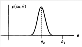
  • Let this probability be $P_i$
    $P_1=p(\text{x};\theta_1)d\text{x}\;\text{and}\;P_2=p(\text{x};\theta_2)d\text{x}$
  • If $P_i$ is small..
    • It says you actually got a data set that unlikely to occur!
    • Not a good guess for $\theta_i$!
  • So it is more likely that $\theta = \theta_2$ is the tru value since $P_2 > P_1$

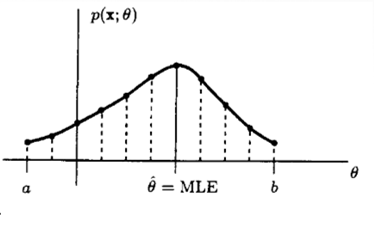
Maximum Likelihood Estimator(MLE)

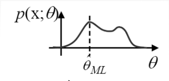
• $\hat\theta_{ML}$ is the value of $\theta$ that maximizes the Likelihood Function, $p(\text{x};\theta)$

  $\hat\theta_{ML}=\arg\max_\theta p(x;\theta)\\ =\arg\max_\theta\ln p(x;\theta)$

• Note : Equivalently, maximizes the log-likelihood function $\ln (p(x;\theta))$

• General Analytical Procedure to Find the MLE
  

  1. Find log-likelihood function : $\ln (p(x;\theta))$
  2. Differentiate w.r.t. $\theta$ and set to 0 : $\partial\ln(p(x;\theta))/\partial\theta=0$
  3. Solve for $\theta$ value that satisfies the equation

     We are still discussing Classical estimation($\theta$ is not a random variable)

     • Bayesian MLE is $\theta$ that maximizes $p(x|\theta)$ with a prior probability $p(\theta)$
     • While MAP estimator maximizes $p(\theta|x)$ Chap. 11

MLE Example

• Same example : DC Level in WGN w/ unknown variance
  (Either CRLB theorem or RBLS theorem is not applicable)
  $p(\text{x};A)=\frac{1}{(2\pi A)^{N/2}}\exp\left[-\frac{1}{2A}\sum_{n=0}^{N-1}(x[n]-A)^2\right]\\[0.3cm] \frac{\partial \ln p(\text{x};A)}{\partial A}=-\frac{N}{2A}+\frac{1}{A}\sum_{n=0}^{N-1}(x[n]-A)+\frac{1}{2A^2}\sum_{n=0}^{N-1}(x[n]-A)^2$
• And $\hat A$ is the value of $A$ that makes it 0
• Replacing $A$ by $\hat A$
  $-\frac{N}{2\hat{A}} + \frac{1}{\hat{A}} \sum_{n=0}^{N-1} x[n] - N + \frac{1}{2\hat{A}^2} \sum_{n=0}^{N-1} x^2[n] - \frac{1}{\hat{A}} \sum_{n=0}^{N-1} x[n] + \frac{N}{2} = 0\\[0.3cm] \Rightarrow \hat{A}^2 + \hat{A} - \frac{1}{N} \sum_{n=0}^{N-1} x^2[n] = 0\\[0.3cm] \Rightarrow \left( \hat{A} + \frac{1}{2} \right)^2 = \frac{1}{N} \sum_{n=0}^{N-1} x^2[n] + \frac{1}{4}\\[0.3cm] \Rightarrow \hat{A} = -\frac{1}{2} + \sqrt{\frac{1}{4} + \frac{1}{N} \sum_{n=0}^{N-1} x^2[n] }$

  Finally, we check the second derivative to determine if it is a maximum or a minimum

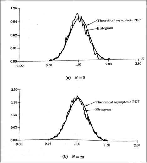
Properties of the MLE

• The example MLE is asymptotically, Unbiased, Efficient(i.e. achieves CRLB) and had a Gaussian PDF
  $\hat \theta \sim ^a\mathcal{N}(\theta,I^{-1}(\theta))$
• If a truly efficient estimator exists, then the ML procedure finds it!
• Use
  $\hat \theta\rightarrow 0=\frac{\partial\ln p(\text{x};\theta)}{\partial\theta}=I(\theta)(g(\text{x})-\theta)$

  If $\partial\ln p(x;\theta)/\partial\theta \rightarrow 0$ then achieve CRLB

• Theorem : Asymptotic properties of the MLE
  • If the PDF $p(\text{x};\theta)$ of the data $\text{x}$ satisfies some regularity conditions, then the MLE of the unknown parameter $\theta$ is asymptotically distributed (for large data records) according to
    $\hat \theta_{ML}\sim^a\mathcal{N}(\theta, I^{-1}(\theta))\\[0.2cm] \text{Regularity : }E\left[\frac{\partial\ln p(x;\theta)}{\partial\theta}\right]=0$
    where $I(\theta)$ is the Fisher information evaluated at the true value of $\theta$, the unknown parameter
  • Regularity condition : existence of the derivatives of the log-likelihood function and nonzero Fisher information
  • Related to Central limit theorem

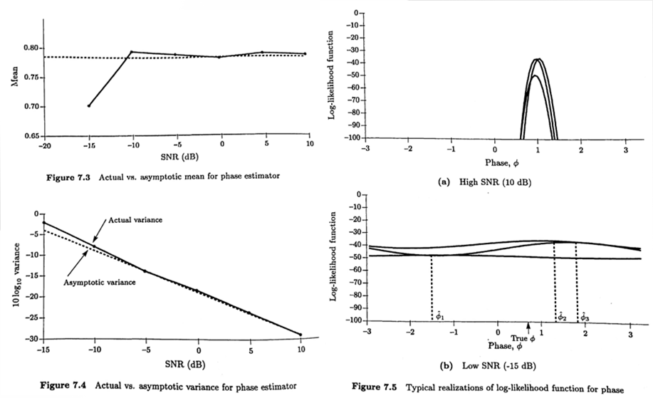
Monte Carlo Simulations(Appendix 7A)

• A methodology for doing computer simulations to evaluate performance of any estimation method illustrate for deterministic signal $s[n;\theta]$ in AWGN
• Monte Carlo Simulation :
  1. Select a particular true parameter value, $\theta_{true}$
     Often interested in doing this for a variety of values of $\theta$, so you would run one MC simulation for each $\theta$ value of interest
  2. Generate signal having true $\theta:s[n;\theta_t]$
  3. Generate WGN having unit variance, $w=\text{randn}(\text{size}(s))$
  4. Form measured data : $x=s+\text{sigma}*w$
     • Choose $\sigma$ to get the desired SNR
     • Usually want to run at many SNR values → do one MC simulation for each SNR value
  5. Compute estimate from data $x$
  6. Repeat steps 3-5 $M$ times
  7. Store all $M$ estimates in a vector EST (assumes scalar $\theta$)
• Statistical Evaluation :
  1. Compute bias
  2. Compute error RMS
  3. Compute the error Variance
  4. Plot Histogram or Scatter Plot (if desired)
• Explore (via plots) how : Bias, RMS, and VAR vary with : $\theta$ value, SNR value, $N$ value, etc.
• DC Level in WGN(Asymptotic properties of the MLE)
  
  $A=1\\\;E[\hat A]\rightarrow A=1\\ \text{var}[\hat A]=\frac{2\beta}{N}=\frac{1}{\text{CRLB}},(N=1)$
  If $N$ get bigger 4 times, std → 1/2, var → 1/4

Example : Phase Estimation in WGN

• MLE of the sinusoidal phase in WGN
  $x[n]=A\cos(2\pi f_0n+\phi+w[n]),\;n=0,1,\cdots,N-1\\[0.2cm] A,f_0,\sigma^2:\text{known},\;w[n]:\text{WGN}$
• All methods for finding the MVUE will fail! → So... Try MLE
• Jointly sufficient statistics
  $T_1(\text{x})=\sum_{n=0}^{N-1}x[n]\cos2\pi f_0n,\;T_2(\text{x})=\sum_{n=0}^{N-1}x[n]\sin 2\pi f_0n$
• MLE : $\phi$ that maximizes
  $p(\mathbf{x}; \phi) = \frac{1}{(2\pi\sigma^2)^{N/2}} \exp\left( -\frac{1}{2\sigma^2} \sum_{n=0}^{N-1} \left[ x[n] - A \cos(2\pi f_0 n + \phi) \right]^2 \right)$
• or minimize
  $J(\phi) = \sum_{n=0}^{N-1} \left[ x[n] - A \cos(2\pi f_0 n + \phi) \right]^2$
• Then
  $\frac{\partial J(\phi)}{\partial \phi} = 2 \sum_{n=0}^{N-1} \left[ x[n] - A \cos(2\pi f_0 n + \phi) \right] A \sin(2\pi f_0 n + \phi) = 0 \\[0.3cm] \Rightarrow \sum_{n=0}^{N-1} x[n] \sin(2\pi f_0 n + \hat{\phi}) = A \sum_{n=0}^{N-1} \sin(2\pi f_0 n + \hat{\phi}) \cos(2\pi f_0 n + \hat{\phi})$
• Where for $f_0$ not near $0$ or $1/2$
  $\frac{1}{N} \sum_{n=0}^{N-1} \sin(2\pi f_0 n + \hat{\phi}) \cos(2\pi f_0 n + \hat{\phi}) = \frac{1}{2N} \sum_{n=0}^{N-1} \sin(4\pi f_0 n + 2\hat{\phi}) \approx 0\\[0.3cm] \Rightarrow \left( \sum_{n=0}^{N-1} x[n] \sin 2\pi f_0 n \right) \cos \hat{\phi} = -\left( \sum_{n=0}^{N-1} x[n] \cos 2\pi f_0 n \right) \sin \hat{\phi}$
• Therefore
  $\hat\phi=-\arctan\frac{\sum_{n=0}^{N-1}x[n]\sin2\pi f_0n}{\sum_{n=0}^{N-1}x[n]\cos2\pi f_0n}=\frac{T_2(x)}{T_1(x)}$
• MLE is function of the sufficient statistics since,
  $p(\text{x};\theta)=g(T_1(\text{x}),T_2(\text{x}),\cdots,T_r(\text{x}),\theta)h(\text{x})$
• Asymptotic PDF of the estimator
  $\hat \phi\sim\mathcal{N}\left(\phi,I^{-1}(\phi)\right)$
  where $I(\phi)=\frac{NA^2}{2\sigma^2}$
• Variance
  $\text{var}(\hat{\phi}) = \frac{1}{N \eta}, \quad \text{where } \eta = \frac{A^2 / 2}{\sigma^2} \text{ is the SNR}\\[0.3cm] 10 \log_{10} \text{var}(\hat{\phi}) = 10 \log_{10} \frac{1}{N \eta} = -10 \log_{10} N - 10 \log_{10} \eta$
  

MLE for Transformed Parameters

• Given PDF $p(\text{x};\theta)$ but want an estimate of $\alpha = g(\theta)$

• What is the MLE for $\alpha$?

  • Two cases :

    • $\alpha=g(\theta)$ is a one-to-one function

      $\hat \alpha_{ML} \text{ maximizes }p(\text{x};g^{-1}(\alpha))$

      

    • $\alpha = g(\theta)$ is not a one-to-one function

      Need to define modified likelihood function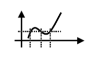

      $\bar p_T(\text{x};\alpha)=\max_{\{\theta;\alpha=g(\theta)\}}p(\text{x};\theta)\\[0.3cm] \hat \alpha_{ML} \text{ maximizes }\bar p_T(\text{x};\alpha)$

      

Example 1

• Example) Transformed DC Level in WGN
  $x[n]=A+w[n],\;n=0,1,\cdots,N-1\\[0.3cm] p(\text{x};A)=\frac{1}{(2\pi\sigma^2)^{N/2}}\exp\left[-\frac{1}{2\sigma^2}\sum_{n=0}^{N-1}(x[n]-A)^2\right],\;-\infty<A<\infty$
• Wish to find the MLE of $\alpha = \exp(A)$
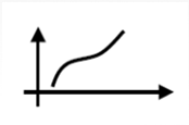
  $p_T(\text{x};\alpha)=\frac{1}{(2\pi\sigma^2)^{N/2}}\exp\left[-\frac{1}{2\sigma^2}\sum_{n=0}^{N-1}(x[n]-\ln \alpha)^2\right],\;\alpha>0$
• Maximizing $p_T(\text{x};\alpha)$ results in
  $\sum_{n=0}^{N-1}(x[n]-\ln\hat\alpha)\frac{1}{\hat\alpha}=0\rightarrow\hat\alpha\\[0.3cm] \hat\alpha=\exp(\bar x)=\exp(\hat A)$
• The MLE of the transformed parameter is the transform of the MLE of the original parameter

  Invariance property

Example 2

• Transformed DC Level in WGN, $\alpha=A^2\rightarrow A=\pm\sqrt \alpha$ : not one-to-one
  $p_{T_1}(\mathbf{x}; \alpha) = \frac{1}{(2\pi\sigma^2)^{N/2}} \exp \left[ -\frac{1}{2\sigma^2} \sum_{n=0}^{N-1} \left( x[n] - \sqrt{\alpha} \right)^2 \right], \quad \alpha \geq 0\\[0.3cm] p_{T_2}(\mathbf{x}; \alpha) = \frac{1}{(2\pi\sigma^2)^{N/2}} \exp \left[ -\frac{1}{2\sigma^2} \sum_{n=0}^{N-1} \left( x[n] + \sqrt{\alpha} \right)^2 \right], \quad \alpha > 0$
• The MLE of $\alpha$ is the value that maximizes the maximum between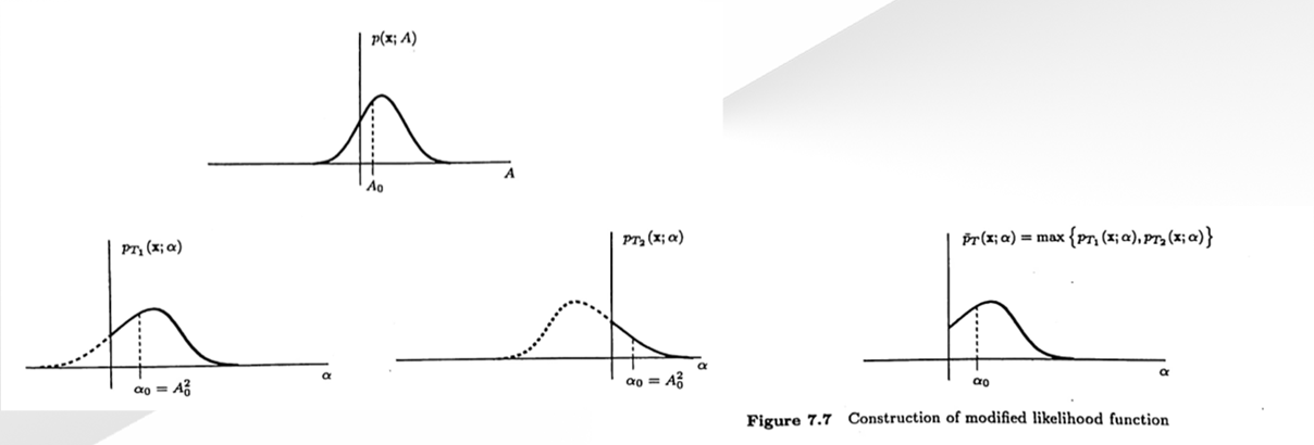 $p_{T_1}(\text{x};\alpha)$ and $p_{T_2}(\text{x};\alpha)$
  $\hat \alpha=\arg\max_{\alpha\geq0}\{p_{T_1}(\text{x};\alpha),p_{T_2}(\text{x};\alpha)\}\\[0.2cm] \rightarrow\hat\alpha=\arg\max_{\alpha\geq0}\{p(\text{x};\sqrt\alpha),p(\text{x};-\sqrt\alpha\}\\[0.2cm] =\left[\arg\max_{\sqrt\alpha\geq0}\{p(\text{x};\sqrt\alpha),p(\text{x};-\sqrt\alpha)\}\right]^2\\[0.2cm] =\left[\arg\max_A p(\text{x};A)\right]^2=\hat A^2=\bar x^2$
  

Invariance Property of MLE

• Theorem : Invariance property of the MLE
  • If parameter $\theta$ is mapped according to $\alpha =g(\theta)$ then the MLE of $\alpha$ is given by
    $\hat \alpha =g(\hat\theta)$
    where $\hat\theta$ is the MLE of $\theta$, found by maximizing $p(\text{x};\theta)$

    If $g(\theta)$ is not a one-to-one function, then $\hat\alpha$ maximizes the modified likelihood function $\bar p_T(\text{x};\alpha)$, defined as

    $\bar p_T(\text{x};\alpha)=\max_{\{\theta:\alpha=g(\theta)\}}p(\text{x};\theta)$

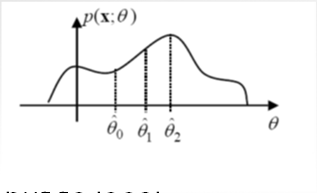
Numerical Determination of the MLE

• In all previous examples we ended up with a closed-form expression for the MLE
  $\hat\theta_{ML}=f(\text{x})$
• Numerical determination of the MLE
  A distint advantage of the MLE is that we can find it for a given data set numerically
• For a finite interval - grid search
• But... For the parameters that span infinite interval
  1. Newton-Raphson method
  2. Scoring approach
  3. Expectation-Maximization(EM) algorithm

     Iterative methods ▷ will result in local maximum ▷ good initial guess is important

• For the parameters that can span infinite interval - iterative method
  

  • Step 1 : Pick some initial estimate $\hat\theta_0$
  • Step 2 : Iteratively improve it using
    $\hat\theta_{k+1}=f(\hat\theta_k,\text{x})\text{ such that}\\[0.2cm] \lim_{k\rightarrow\infty} p(\text{x};\theta_k)=\max_\theta p(\text{x};\theta)$

• Convergence Issues : May not converge, or may converge, but to local maximum

  Good initial guess is needed
  (Use rough grid search to initialize or multiple initialization)

Exponential in WGN Example

• Estimate $r$
  $x[n]=r^n+w[n],\;n=0,1,\cdots,N-1\\[0.2cm] E[x[n]]=r^n\\[0.2cm] \rightarrow p(\text{x};r)=\frac{1}{(2\pi\sigma^2)^{N/2}}\exp\left[-\frac{1}{2\sigma^2}\sum_{n=0}^{N-1}(x[n]-r^n)^2\right]$
• To find MLE
  $\frac{\partial \ln p(\text{x};\theta)}{\partial\theta}=0\\[0.3cm] \rightarrow \sum_{n=0}^{N-1}(x[n]-r^n)nr^{n-1}=0:\text{can't be solved directly}$
• Iterative method : Newton-Raphson method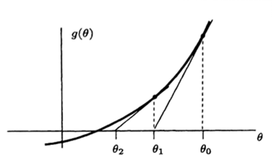
  $g(\theta) = \frac{\partial \ln p(\mathbf{x}; \theta)}{\partial \theta} = 0 \Rightarrow g(\theta) \approx g(\theta_0) + \left. \frac{dg(\theta)}{d\theta} \right|_{\theta = \theta_0} (\theta - \theta_0)\\[0.3cm] \theta_1 = \theta_0 - \frac{g(\theta_0)}{\left. \frac{dg(\theta)}{d\theta} \right|_{\theta = \theta_0}} \Rightarrow \theta_{k+1} = \theta_k - \frac{g(\theta_k)}{\left. \frac{dg(\theta)}{d\theta} \right|_{\theta = \theta_k}}\\[0.3cm] \Rightarrow \theta_{k+1} = \theta_k - \left[ \frac{\partial^2 \ln p(\mathbf{x}; \theta)}{\partial \theta^2} \right]^{-1} \left. \frac{\partial \ln p(\mathbf{x}; \theta)}{\partial \theta} \right|_{\theta = \theta_k}$
  
• The iteration may not converge
• Even if the iteration converges, the point found may not be the global maximum but possibly only a local maximum or even a local minimum

  Good initial guess is important

  $\frac{\partial \ln p(\mathbf{x}; r)}{\partial r} = \frac{1}{\sigma^2} \sum_{n=0}^{N-1} \left( x[n] - r^n \right) n r^{n-1}\\[0.3cm] \frac{\partial^2 \ln p(\mathbf{x}; r)}{\partial r^2} = \frac{1}{\sigma^2} \left[ \sum_{n=0}^{N-1} n(n-1) x[n] r^{n-2} - \sum_{n=0}^{N-1} n(2n-1) r^{2n-2} \right]\\[0.3cm] = \frac{1}{\sigma^2} \sum_{n=0}^{N-1} n r^{n-2} \left[ (n-1) x[n] - (2n-1) r^n \right]\\[0.3cm] I(r)=-E\left[\frac{\partial^2\ln p(x;r)}{\partial r^2}\right]\\[0.3cm] \Rightarrow r_{k+1} = r_k - \frac{\sum_{n=0}^{N-1} n r_k^{n-2} \left( (n-1) x[n] - (2n-1) r_k^n \right)}{\sum_{n=0}^{N-1} n r_k^{n-2} \left[ (n-1) x[n] - (2n-1) r_k^n \right]}$

---

• Iterative method : the method of scoring
• Motivation :
  $\frac{\partial^2 \ln p(\mathbf{x}; \theta)}{\partial \theta^2} \Bigg|_{\theta = \theta_k} \approx -I(\theta_k)$
• For IID samples, by the law of large numbers
  $\frac{\partial^2 \ln p(\mathbf{x}; \theta)}{\partial \theta^2} = \sum_{n=0}^{N-1} \frac{\partial^2 \ln p(x[n]; \theta)}{\partial \theta^2} = N \left( \frac{1}{N} \sum_{n=0}^{N-1} \frac{\partial^2 \ln p(x[n]; \theta)}{\partial \theta^2} \right)\\[0.3cm] \approx N E\left[ \frac{\partial^2 \ln p(x[n]; \theta)}{\partial \theta^2} \right] = -N i(\theta) = -I(\theta)$
• The method of scoring
  $\theta_{k+1} = \theta_k + I^{-1}(\theta) \left. \frac{\partial \ln p(\mathbf{x}; \theta)}{\partial \theta} \right|_{\theta = \theta_k}$

  The expectation provides more stable iteration

  $I(r) = \frac{1}{\sigma^2} \sum_{n=0}^{N-1} n^2 r^{2n-2}\\[0.3cm] \Rightarrow r_{k+1} = r_k + \frac{\sum_{n=0}^{N-1} \left( x[n] - r_k^n \right) n r_k^{n-1}}{\sum_{n=0}^{N-1} n^2 r_k^{2n-2}}$

MLE for a Vector Parameter

• $\hat\theta_{ML}$ is the vector that satifies
  $\frac{\partial \ln p(\text{x};\theta}{\partial\theta}=0$
• Example : DC Level in AWGN with unknown noise variance
  $x[n]=A+w[n],\;n=0,1,\cdots,N-1\\[0.2cm] \theta=[A\sigma^2]^T\\[0.2cm] \frac{\partial \ln p(\mathbf{x}; \theta)}{\partial A} = \frac{1}{\sigma^2} \sum_{n=0}^{N-1} (x[n] - A)\\[0.2cm] \frac{\partial \ln p(\mathbf{x}; \theta)}{\partial \sigma^2} = -\frac{N}{2\sigma^2} + \frac{1}{2\sigma^4} \sum_{n=0}^{N-1} (x[n] - A)^2\\[0.2cm]\\[0.2cm] \rightarrow \hat A=\bar x,\\[0.3cm] \hat{\sigma}^2 = \frac{1}{N} \sum_{n=0}^{N-1} (x[n] - \bar{x})^2$

Asymptotic Properties of Vector MLE

• Theorem : Asymptotic properties of the MLE (vector parameter)
  • If the PDF $p(\text{x};\theta)$ of the data $\text{x}$ satisfies some regularity conditions,
  • Then the MLE of the unknown parameter $\theta$ is asymptotically distributed(for large data records) according to
    $\hat\theta\sim^a\mathcal{N}(\theta,I^{-1}(\theta))$
    where $I(\theta)$ is the Fisher information matrix evaluated at the true value of the unknown parameter
• So the vector ML is asymptotically unbiased and efficient
• Invariance Property Holds for Vector Case
  $\alpha=g(\theta),\text{ then }\hat\alpha_{ML}=g(\hat\theta_{ML})$
• Example : DC Level in AWGN with unknown noise variance
  $\bar x \sim\mathcal{N}(A,\frac{\sigma^2}{N})\\[0.3cm] T=\sum_{n=0}^{N-1}\frac{(x[n]-\bar x)^2}{\sigma^2} \sim\chi^2_{N-1}$
  and mutually independent
  • For large $N$, by central limit theorem
    $\chi^2_N \sim a\mathcal{N}(N, 2N) \quad \Rightarrow \quad T \sim a\mathcal{N}(N-1, 2(N-1))$
    or
    $E(\hat{\theta}) = \begin{bmatrix} \frac{A}{N} \\ \frac{(N-1)\sigma^2}{N} \end{bmatrix} \Rightarrow \begin{bmatrix} A \\ \sigma^2 \end{bmatrix} = \theta, \\[0.3cm] C(\theta) = \begin{bmatrix} \frac{\sigma^2}{N} & 0 \\ 0 & \frac{2(N-1)\sigma^4}{N^2} \end{bmatrix} \Rightarrow \begin{bmatrix} \frac{\sigma^2}{N} & 0 \\ 0 & \frac{2\sigma^4}{N} \end{bmatrix} = I^{-1}(\theta)$

Expectation-Maximization Algorithm

1. Newton-Raphson method
2. Scoring approach
3. Expectation-Maximization(EM) algorithm
   1. Increase the likelihood at each step
   2. Guaranteed to converge under mild conditions(to at least a local maximum)
   3. Uses complete and incomplete data concepts
   4. Good for complicated multi-parameter cases

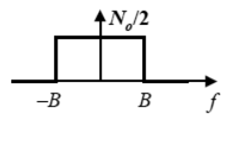
• Example : Multiple frequencies in WGn
  $x[n]=\sum_{i=1}^p \cos2\pi f_in+w[n],\;n=0,1,\cdots,N-1$
  • $w[n]$ : WGN
  • Variance $\sigma^2$
  • $\mathbf{f} = \begin{bmatrix} f_1 & f_2 & \dots & f_p \end{bmatrix}^T$ : parameter to estimate
  • Objective function to minimize :
    $J(\mathbf{f}) = \sum_{n=0}^{N-1} \left( x[n] - \sum_{i=1}^{p} \cos(2\pi f_i n) \right)^2$
  • If the original data could be replaced by the independent data sets
    $y_i[n]=\cos2\pi f_in+w_i[n],\;n=0,1,\cdots,N-1,\;i=1,2,\cdots,p$
    where $w_i[n]$ is WGN with variance $\sigma_i^2$, then the problem would be decoupled
  • Decoupled objective function to minimize :
    $J(f_i) = \sum_{n=0}^{N-1} \left( y_i[n] - \cos 2\pi f_i n \right)^2, \quad i = 1, 2, \dots, p$
    $p-D$ minimization reduced to $p$ seperate 1-D minimization
  • The new data set $\{y_1[n],y_2[n],\cdots,y_p[n]\}$ : complete data
  • $x[n]$ : original or incomplete data
    $x[n] = \sum_{i=1}^{p} y_i[n], \quad w[n] = \sum_{i=1}^{p} w_i[n], \quad \sigma^2 = \sum_{i=1}^{p} \sigma_i^2$
  • The decomposition is not unique :
    $x[n]=y_1[n]+y_2[n],\;y_1[n]=\sum_{i=1}^p\cos2\pi f_in,\;y_2[n]=w[n]$

Expectation-Maximization Algorithm - General

• Suppose that there is a complete to incomplete data transformation
  $\text{x}=g(y_1,y_2,\cdots,y_M)=g(y)$, where $g$ is a many-to-one transformation
• MLE : $\theta$ that maximizes $\ln p_x(\text{x};\theta)$
• EM algorithm : maximize $\ln p_y(y;\theta)$, but $y$ is not available, so maximize
  $E_{y|x}[\ln p_y(y;\theta)]=\int\ln p_y(y;\theta)p(y|x;\theta)dy$
  • Expectation (E) Step : Determine the average log-likelihood the complete data
    $U(\theta,\theta_k)=\int\ln p_y(y;\theta)p(y|x;\theta_k)dy$
  • Maximization (M) Step : Maximize the average log-likelihood function of the complete data
• Example : Multiple frequencies in WGN
  • Expectation (E) Step : For $i=1,2,\cdots,p$
    $\hat y_i[n]=\cos2\pi f_{i_k}n+\beta_i\left(x[n]-\sum_{i=1}^p\cos2\pi f_{i_k}n\right)$
  • Maximization (M) Step : For $i=1,2,\cdots,p$
    $f_{i_{k+1}}=\arg\max_{f_i}\sum_{n=0}^{N-1}\hat y_i[n]\cos 2\pi f_i n$
    where $\beta_i$'s can be arbitrarily chosen as long as $\sum_{i=1}^p\beta_i=1$

MLE Example - Range Estimation

• Transmit pulse $s(t)$, nonzero over $t\in[0,T_s]$
• Receive reflection $s(t-\tau_0)$
• Estimation of time delay $\tau_0$, since the round trip delay $\tau_0=2R/c$
• Continuous time signal model
  $x(t)=s(t-\tau_0)+w(t),\;0\leq t\leq T=T_s+\tau_{0_\text{max}}$
• Discrete time signal model
  • Sample every $\triangle=1/(2B)$ sec, $x[n]=s(n\triangle-\tau_0)+w[n],\;n=0,1,\cdots, N-1$
  • $s(n\triangle-\tau_0)$ has $M$ non-zero samples starting at $n_0$
    $x[n] = \begin{cases} w[n], & 0 \leq n \leq n_0 - 1 \\ s(n\Delta - \tau_0) + w[n], & n_0 \leq n \leq n_0 + M - 1 \\ w[n], & n_0 + M \leq n \leq N - 1 \end{cases}$

    PSD of $w(t)$	ACF of $w(t)$

  • $r_{ww}(\tau)=N_0B\frac{\sin2\pi\tau B}{2\pi \tau B}$
• Range Estimation Likelihood Function :
  $p(\mathbf{x}; n_0) = \left( \prod_{n=0}^{n_0-1} \frac{1}{\sqrt{2\pi \sigma^2}} \exp\left[ -\frac{x^2[n]}{2\sigma^2} \right] \right) \cdot \left( \prod_{n=n_0}^{n_0+M-1} \frac{1}{\sqrt{2\pi \sigma^2}} \exp\left[ -\frac{(x[n] - s[n-n_0])^2}{2\sigma^2} \right] \right) \\[0.3cm]\cdot \left( \prod_{n=n_0+M}^{N-1} \frac{1}{\sqrt{2\pi \sigma^2}} \exp\left[ -\frac{x^2[n]}{2\sigma^2} \right] \right)\\[0.3cm] = \frac{1}{(2\pi\sigma^2)^{N/2}} \exp\left[ -\frac{1}{2\sigma^2} \sum_{n=0}^{N-1} x^2[n] \right] \\[0.3cm]\cdot \left( \prod_{n=n_0}^{n_0+M-1} \frac{1}{\sqrt{2\pi \sigma^2}} \exp\left[ -\frac{1}{2\sigma^2} \left( -2s[n-n_0]x[n] + s^2[n-n_0] \right) \right] \right)$
• Minimize
  $-2 \sum_{n=n_0}^{n_0+M-1} x[n] s[n-n_0] + \sum_{n=n_0}^{n_0+M-1} s^2[n-n_0]$
• Or, maximize
  $\sum_{n=n_0}^{n_0+M-1} x[n] s[n-n_0]$

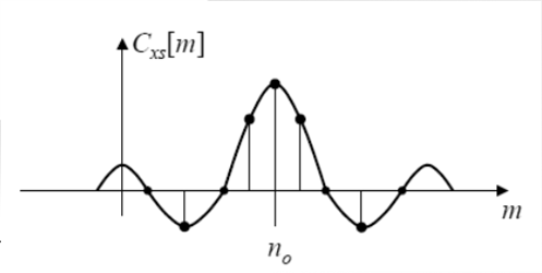
  So, MLE implementation is based on Cross-correlation :
  "Correlate" received signal $x[n]$ with trasmitted signal $s[n]$

• Therefore
  $\hat n_0=\arg\max_{0\leq m\leq N-M}\{C_{XS}[m]\},\\[0.3cm] C_{XS}[m]=\sum_{n=0}^{n-1}x[n]s[n-m]\\[0.3cm] \hat R=(C\triangle/2)\hat n_0$
  • Think of this as an inner product for each $m$
  • Compare data $x[n]$ to all possible delays of signal $s[n]$
    Pick $n_0$ to make them most alike
    

All Content has been written based on lecture of Prof. eui-seok.Hwang in GIST(Detection and Estimation)