machine learning in python
basic flow
import numpy as np
from sklearn.linear_model import LinearRegression
model = LinearRegression() # 모델 정의
model.fit(x, y) # 모델 학습
prediction = model.predict(v) # 값 예측
from sklearn.model_selection import train_test_split# 코드입력
x_train, x_valid, y_train, y_valid = train_test_split(train[feature], train[label], test_size = 0.2, shuffle =True, random_state = 30) # 8 2 비율로 데이터를 training 과 validation으로 나눔목차
- 결측치(imputer) : 빈값 처리
- 이상치
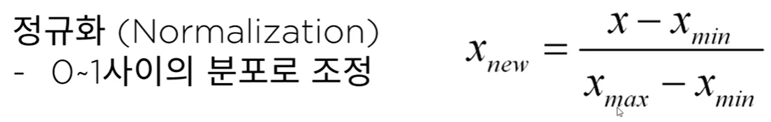
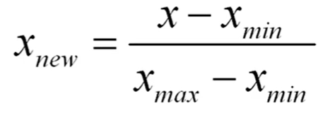
- 정규화(Normalization) : 0~1 사이의 분포로 조정
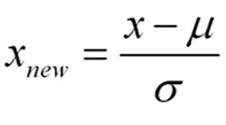
- 표준화(Standardization) : 평균을 0, 표준편차를 1로 맞춤
- 샘플링(over/uder sampling)
- 피처공학(Feature Engineering)
1. 결측치 처리
from sklearn.impute import SimpleImputer

imputer = SimpleImputer(strategy = 'mean') #평균값
imputer = SimpleImputer(strategy= 'most_frequent') #가장 많은 값
train['Embarked'].fillna('S') #이런식으로 수동으로 바꿔줘도 됨

result = imputer.fit_transform(train[['Age', 'Pclass']]) # 학습 및 수정
train[['Age', 'Pclass']].isnull().sum() #null 확인
1-1 . 문자형 데이터 수치형으로 변환
from sklearn.preprocessing import LabelEncoder
train['Sex_num'] = le.fit_transform(train['Sex'])
train['Sex_num'].value_counts() # 0과 1로 변환
1-2 . 온 핫 인코딩
2. 정규화
movie = {'naver': [2, 4, 6, 8, 10],
         'netflix': [1, 2, 3, 4, 5]
         }

from sklearn.preprocessing import MinMaxScaler #정규화 함수
min_max_movie = min_max_scaler.fit_transform(movie)
pd.DataFrame(min_max_movie, columns=['naver', 'netflix'])
3. 표준화
from sklearn.preprocessing import StandardScaler
standard_scaler = StandardScaler()
scaled = standard_scaler.fit_transform(x.reshape(-1, 1) )
round(scaled.mean(), 2), scaled.std() # 평균이 0, 표준편차 1
4. train, validate data 구분
주로 train, test data를 8:2 정도로 분할한다.
from sklearn.model_selection import train_test_split # testing data와 validation data 검증
x_train, x_valid, y_train, y_valid = train_test_split(df_iris.drop('target', 1), df_iris['target'], stratify=df_iris['target']) #stratify를 통해 클래스를 균등하게 배분
machine learning 기법
- Classification
- Regression
- Clustering
1. Classification
1-1. Logistic Regression
로지스틱 회귀(영어: logistic regression)는 영국의 통계학자인 D. R. Cox가 1958년에 제안한 확률 모델
독립 변수의 선형 결합을 이용하여 사건의 발생 가능성을 예측하는데 사용되는 통계 기법
LogisticRegression, 서포트 벡터 머신 (SVM) 과 같은 알고리즘은 이진 분류만 가능합니다. (2개의 클래스 판별만 가능합니다.)
하지만, 3개 이상의 클래스에 대한 판별을 진행하는 경우, 다음과 같은 전략으로 판별하게 됩니다.
one-vs-rest (OvR): K 개의 클래스가 존재할 때, 1개의 클래스를 제외한 다른 클래스를 K개 만들어, 각각의 이진 분류에 대한 확률을 구하고, 총합을 통해 최종 클래스를 판별
one-vs-one (OvO): 4개의 계절을 구분하는 클래스가 존재한다고 가정했을 때, 0vs1, 0vs2, 0vs3, ... , 2vs3 까지 NX(N-1)/2 개의 분류기를 만들어 가장 많이 양성으로 선택된 클래스를 판별
대부분 OvsR 전략을 선호합니다.
from sklearn.model_selection import train_test_split # testing data와 validation data 검증
x_train, x_valid, y_train, y_valid = train_test_split(df_iris.drop('target', 1), df_iris['target'], stratify=df_iris['target']) #stratify를 통해 클래스를 균등하게 배분

from sklearn.linear_model import LogisticRegression
model = LogisticRegression()
model.fit(x_train, y_train)
prediction = model.predict(x_valid) # validation data로 예측
(prediction == y_valid).mean() #평가
1-2. Stochastic Gradient Descent (SGD)
from sklearn.linear_model import SGDClassifier
sgd = SGDClassifier(penalty = 'elasticnet', random_state=0, n_jobs=-1)
# penalty를 통한 overfitting 방지, random state를 통한 seed 고정, n_jobs는 cpu 활용 수 -1의 경우 활용할 수 있는 cpu 모두 사용
다양한 방식으로 하이퍼파라메터를 수정하여 performance를 증가시켜보자
1-3. KNeighbors Classifier (KNN)
from sklearn.neighbors import KNeighborsClassifier
knc = KNeighborsClassifier()
knc_pred = knc.predict(x_valid)
(knc_pred == y_valid).mean()
1-4. Support Vector Machine (SVM)
새로운 데이터가 어느 카테고리에 속할지 판단하는 비확률적 이진 선형 분류 모델을 만듦.
경계로 표현되는 데이터들 중 가장 큰 폭을 가진 경계를 찾는 알고리즘.
LogisticRegression과 같이 이진 분류만 가능합니다. (2개의 클래스 판별만 가능합니다.)
OvsR 전략 사용
from sklearn.svm import SVC
svc=SVC()
svc.fit(x_train, y_train)
svc_pred = svc.predict(x_valid)
(svc_pred == y_valid).mean()
1-5. Decision Tree
from sklearn.tree import DecisionTreeClassifier
dtc = DecisionTreeClassifier()
.
.
.
graph_viz 을 활용하여 decision tree 시각화 하기
from sklearn.tree import export_graphviz
from subprocess import call
def graph_tree(model):
    # .dot 파일로 export 해줍니다
    export_graphviz(model, out_file='tree.dot')

    # 생성된 .dot 파일을 .png로 변환

    call(['dot', '-Tpng', 'tree.dot', '-o', 'decistion-tree.png', '-Gdpi=600'])

    # .png 출력
    return Image(filename = 'decistion-tree.png', width=500)
정확도 함정에 대한 모델 평가 지표
1. 오차행렬(confusionmatrix)
-
정밀도와 재현율
-
f1 score
정밀도와 재현율의 조화 평균을 나타내는 지표
2. Regression
평가지표
- MSE : 예측값과 실제값의 차이에 대한 제곱에 대해 평균
- MAE : 예측값과 실제값의 차이에 대한 절댓값에 대해 평균
- RMSE : MSE에 루트를 씌운것
from sklearn.metrics import mean_absolute_error, mean_squared_error실습용 model 시각화 함수
import matplotlib.pyplot as plt
import seaborn as sns

my_predictions = {}

colors = ['r', 'c', 'm', 'y', 'k', 'khaki', 'teal', 'orchid', 'sandybrown',
          'greenyellow', 'dodgerblue', 'deepskyblue', 'rosybrown', 'firebrick',
          'deeppink', 'crimson', 'salmon', 'darkred', 'olivedrab', 'olive',
          'forestgreen', 'royalblue', 'indigo', 'navy', 'mediumpurple', 'chocolate',
          'gold', 'darkorange', 'seagreen', 'turquoise', 'steelblue', 'slategray',
          'peru', 'midnightblue', 'slateblue', 'dimgray', 'cadetblue', 'tomato'
         ]

def plot_predictions(name_, pred, actual):
    df = pd.DataFrame({'prediction': pred, 'actual': y_test})
    df = df.sort_values(by='actual').reset_index(drop=True)

    plt.figure(figsize=(12, 9))
    plt.scatter(df.index, df['prediction'], marker='x', color='r')
    plt.scatter(df.index, df['actual'], alpha=0.7, marker='o', color='black')
    plt.title(name_, fontsize=15)
    plt.legend(['prediction', 'actual'], fontsize=12)
    plt.show()

def mse_eval(name_, pred, actual):
    global predictions
    global colors

    plot_predictions(name_, pred, actual)

    mse = mean_squared_error(pred, actual)
    my_predictions[name_] = mse

    y_value = sorted(my_predictions.items(), key=lambda x: x[1], reverse=True)

    df = pd.DataFrame(y_value, columns=['model', 'mse'])
    print(df)
    min_ = df['mse'].min() - 10
    max_ = df['mse'].max() + 10

    length = len(df)

    plt.figure(figsize=(10, length))
    ax = plt.subplot()
    ax.set_yticks(np.arange(len(df)))
    ax.set_yticklabels(df['model'], fontsize=15)
    bars = ax.barh(np.arange(len(df)), df['mse'])

    for i, v in enumerate(df['mse']):
        idx = np.random.choice(len(colors))
        bars[i].set_color(colors[idx])
        ax.text(v + 2, i, str(round(v, 3)), color='k', fontsize=15, fontweight='bold')

    plt.title('MSE Error', fontsize=18)
    plt.xlim(min_, max_)

    plt.show()

def remove_model(name_):
    global my_predictions
    try:
        del my_predictions[name_]
    except KeyError:
        return False
    return True
weight 시각화 함수
def plot_coef(columns, coef):
   coef_df = pd.DataFrame(list(zip(columns, coef)))
   coef_df.columns=['feature', 'coef']
   coef_df = coef_df.sort_values('coef', ascending=False).reset_index(drop=True)

   fig, ax = plt.subplots(figsize=(9, 7))
   ax.barh(np.arange(len(coef_df)), coef_df['coef'])
   idx = np.arange(len(coef_df))
   ax.set_yticks(idx)
   ax.set_yticklabels(coef_df['feature'])
   fig.tight_layout()
   plt.show()
Linear Regression
site :
https://scikitlearn.org/stable/modules/generated/sklearn.linear_model.LinearRegression.html
from sklearn.linear_model import LinearRegression
model = LinearRegression(n_jobs= -1) # n_jobs는 cpu 사용 개수
model.fit(x_train, y_train)
pred = model.predict(x_test)
mse_eval('LinearRegression', pred, y_test)
Ridge, Lasso, ElasticNet
Regularization
L2 : 각 가중치 제곱의 합에 규제 강도(Regularization Strength) λ를 곱한다. λ를 크게 하면 가중치가 더 많이 감소되고(규제를 중요시함), λ를 작게 하면 가중치가 증가한다(규제를 중요시하지 않음).
수식 : Error=MSE+αw^2
L1 : 가중치의 제곱의 합이 아닌 가중치의 합을 더한 값에 규제 강도(Regularization Strength) λ를 곱하여 오차에 더한다.
어떤 가중치(w)는 실제로 0이 된다. 즉, 모델에서 완전히 제외되는 특성이 생기는 것이다.
수식 : Error=MSE+α|w|
L2 규제가 L1 규제에 비해 더 안정적이라 일반적으로는 L2규제가 더 많이 사용된다
L2를 사용한 것이 Ridge model L2을 사용한 것이 Lasso model
- Ridge
from sklearn.linear_model import Ridge
alphas = [100, 10, 1, 0.1, 0.01, 0.001, 0.0001] # 값이 커질 수록 큰 규제입니다. 규제가 클 수록 오버피팅이 줄어듬
for alpha in alphas:
    ridge =Ridge(alpha = alpha) # 코드입력
    ridge.fit(x_train, y_train)
    pred = ridge.predict(x_test)
    mse_eval('Ridge(alpha={})'.format(alpha), pred, y_test)
ridge.coef_ #이를 통해 각 weight를 확인 할 수 있음- Lasso
from sklearn.linear_model import Lasso
alphas = [100, 10, 1, 0.1, 0.01, 0.001, 0.0001]
for alpha in alphas:
    lasso = Lasso(alpha = alpha ) # 코드입력
    lasso.fit(x_train, y_train)
    pred = lasso.predict(x_test)
    mse_eval('Lasso(alpha={})'.format(alpha), pred, y_test)
규제를 주면 줄수록 퍼모먼스가 떨어지는 모델
- ElasticNet
Ridge와 Lasso의 융합 (L2와 L1의 적절한 혼합)
from sklearn.linear_model import ElasticNet
ratios = [0.2, 0.5, 0.8]
for ratio in ratios:
    elasticnet = ElasticNet(alpha = 0.5, l1_ratio=ratio) # alpha는 그냥 0.5로 고정 시킴
    elasticnet.fit(x_train, y_train)
    pred = elasticnet.predict(x_test)
    mse_eval('ElasticNet(l1_ratio={})'.format(ratio), pred, y_test)
Scaler
각 feature의 값마다 scale이 다르기 때문에 이를 맞춰줄 필요가 있다.
전처리의 일종으로 실제 data들을 feature간의 값의 차이가 크고 outlier가 많기 때문에 꼭 scaling을 하는 것이 좋다.
#평균(mean)을 0, 표준편차(std)를 1로 만들어 주는 스케일러
from sklearn.preprocessing import StandardScaler, MinMaxScaler, RobustScaler
std_scaler = StandardScaler()
std_scaled = std_scaler.fit_transform(x_train)

# min값과 max값을 0~1사이로 정규화
minmax_scaler = MinMaxScaler()
minmax_scaled = minmax_scaler.fit_transform(x_train)

#중앙값(median)이 0, IQR(interquartile range)이 1이 되도록 변환. outlier 값 처리에 유용
robust_scaler = RobustScaler()
robust_scaled = robust_scaler.fit_transform(x_train)
round(pd.DataFrame(robust_scaled).median(), 2)
Pipeline
from sklearn.pipeline import make_pipeline
elasticnet_pipeline = make_pipeline(
    StandardScaler(), ElasticNet(alpha = 0.1, l1_ratio= 0.2)
)# pipeline이라는 내부 함수를 통해 scaler를 쉽게 변경하면서 model testing이 가능하다.

elasticnet_pred = elasticnet_pipeline.fit(x_train, y_train).predict(x_test)
mse_eval('Standard ElasticNet', elasticnet_pred, y_test)
Polynomial Features
다항식의 계수간 상호작용을 통해 새로운 feature를 생성합니다.
예를들면, [a, b] 2개의 feature가 존재한다고 가정하고,
degree=2로 설정한다면, polynomial features 는 [1, a, b, a^2, ab, b^2] 가 됩니다.
feature들 간의 교효작용의 여지를 파악하여 새로운 변수들을 만들어냄, 이를 통해 feature간의 상호작용을 고려한 model을 설계 할 수 있음 하지만 변수가 많다고 해서 꼭 좋은 것만은 아님, 불필요한 변수는 제거하는 것이 학습에 더 도움이 됨
from sklearn.preprocessing import PolynomialFeatures
poly_pipeline = make_pipeline(
    PolynomialFeatures(degree=2, include_bias= False), StandardScaler(), ElasticNet(alpha=0.1, l1_ratio=0.2)
    )
poly_pred= poly_pipeline.fit(x_train, y_train).predict(x_test)
mse_eval('Poly Elastic', poly_pred, y_test)
3. Clusgtering
4. Ensemble
scikit-learn site
https://scikit-learn.org/stable/modules/classes.html?highlight=ensemble#module-sklearn.ensemble
머신러닝 앙상블이란 여러개의 머신러닝 모델을 이용해 최적의 답을 찾아내는 기법이다. 여러 모델을 이용하여 데이터를 학습하고, 모든 모델의 예측결과를 평균하여 예측
앙상블 기법의 종류
Voting은 단어 뜻 그대로 투표를 통해 결정하는 방식입니다. Voting은 Bagging과 투표방식이라는 점에서 유사하지만, 다음과 같은 큰 차이점이 있습니다. 다시 말하자면 Voting은 여러 알고리즘의 조합에 대한 앙상블
Bagging은 하나의 단일 알고리즘에 대하여 여러 개의 샘플 조합으로 앙상블
1. 보팅 (Voting):
Voting은 다른 알고리즘 model을 조합해서 사용합니다.
from sklearn.ensemble import VotingRegressor, VotingClassifier

single_models = [
    ('linear_reg', linear_reg),
    ('ridge', ridge),
    ('lasso', lasso),
    ('elasticnet_pipeline', elasticnet_pipeline),
    ('poly_pipeline', poly_pipeline)
]

voting_regressor = VotingRegressor(single_models, n_jobs=-1)
voting_regressor.fit(x_train, y_train)
voting_pred = voting_regressor.predict(x_test)
mse_eval('Voting Ensemble', voting_pred, y_test)

from sklearn.ensemble import VotingClassifier
from sklearn.linear_model import LogisticRegression, RidgeClassifier
models = [
    # 코드입력
]
vc = VotingClassifier(models, voting='hard')
2. 배깅 (Bagging):
Bagging은 같은 알고리즘 내에서 다른 sample 조합을 사용합니다.
Bagging은 Bootstrap Aggregating의 줄임말입니다.
Bootstrap = Sample(샘플) + Aggregating = 합산
Bootstrap은 여러 개의 dataset을 중첩을 허용하게 하여 샘플링하여 분할하는 방식
데이터 셋의 구성이 [1, 2, 3, 4, 5 ]로 되어 있다면,
group 1 = [1, 2, 3]
group 2 = [1, 3, 4]
group 3 = [2, 3, 5]
대표적인 Bagging ensemble
1. Randomforest : decisiontree 기반의 bagging
구현하기 쉬우면서도 성능이 매우 뛰어남
from sklearn.ensemble import RandomForestRegressor, RandomForestClassifier
rfr = RandomForestRegressor() # 코드입력
rfr.fit(x_train, y_train)
rfr_pred = rfr.predict(x_test)
mse_eval('RandomForest Ensemble', rfr_pred, y_test)
주요 Hyperparameter
random_state: 랜덤 시드 고정 값. 고정해두고 튜닝할 것!
n_jobs: CPU 사용 갯수
max_depth: 깊어질 수 있는 최대 깊이. 과대적합 방지용
n_estimators: 앙상블하는 트리의 갯수
max_features: 최대로 사용할 feature의 갯수. 과대적합 방지용
min_samples_split: 트리가 분할할 때 최소 샘플의 갯수. default=2. 과대적합 방지용
rfr = RandomForestRegressor(random_state=42, n_estimators=1000, max_depth=7, max_features = 0.8)# 코드입력
rfr.fit(x_train, y_train)
rfr_pred = rfr.predict(x_test)
mse_eval('RandomForest Ensemble w/ Tuning', rfr_pred, y_test)
3. 부스팅 (Boosting): 이전 오차를 보완하면서 가중치 부여
약한 학습기를 순차적으로 학습을 하되, 이전 학습에 대하여 잘못 예측된 데이터에 가중치를 부여해 오차를 보완해 나가는 방식입니다.
장점 : 성능이 매우 우수하다 (Lgbm, XGBoost)
단점 : 부스팅 알고리즘의 특성상 계속 약점(오분류/잔차)을 보완하려고 하기 때문에 잘못된 레이블링이나 아웃라이어에 필요 이상으로 민감할 수 있다
다른 앙상블 대비 학습 시간이 오래걸린다는 단점이 존재
대표적인 Boosting 앙상블
1. AdaBoost
2. GradientBoost
3. LightGBM (LGBM)
4. XGBoost
1. GradientBoost
성능이 우수함, 학습시간이 해도해도 너무 느리다
주요 Hyperparameter
random_state: 랜덤 시드 고정 값. 고정해두고 튜닝할 것!
n_jobs: CPU 사용 갯수
learning_rate: 학습율. 너무 큰 학습율은 성능을 떨어뜨리고, 너무 작은 학습율은 학습이 느리다. 적절한 값을 찾아야함. n_estimators와 같이 튜닝. default=0.1
n_estimators: 부스팅 스테이지 수. (랜덤포레스트 트리의 갯수 설정과 비슷한 개념). default=100
subsample: 샘플 사용 비율 (max_features와 비슷한 개념). 과대적합 방지용
min_samples_split: 노드 분할시 최소 샘플의 갯수. default=2. 과대적합 방지용
from sklearn.ensemble import GradientBoostingRegressor, GradientBoostingClassifier
gbr = GradientBoostingRegressor(random_state=42, learning_rate =0.01)# 코드입력
gbr.fit(x_train, y_train)
gbr_pred = gbr.predict(x_test)
mse_eval('GradientBoost Ensemble (lr=0.01)', gbr_pred, y_test)
2. XGBoost (eXtreme Gradient Boosting)
scikit-learn 패키지가 아닙니다.
성능이 우수함
GBM보다는 빠르고 성능도 향상되었습니다.
여전히 학습시간이 매우 느리다
주요 Hyperparameter
random_state: 랜덤 시드 고정 값. 고정해두고 튜닝할 것!
n_jobs: CPU 사용 갯수
learning_rate: 학습율. 너무 큰 학습율은 성능을 떨어뜨리고, 너무 작은 학습율은 학습이 느리다. 적절한 값을 찾아야함. n_estimators와 같이 튜닝. default=0.1
n_estimators: 부스팅 스테이지 수. (랜덤포레스트 트리의 갯수 설정과 비슷한 개념). default=100
max_depth: 트리의 깊이. 과대적합 방지용. default=3.
subsample: 샘플 사용 비율. 과대적합 방지용. default=1.0
max_features: 최대로 사용할 feature의 비율. 과대적합 방지용. default=1.0
from xgboost import XGBRegressor, XGBClassifier
xgb = XGBRegressor(random_state=42, learning_rate=0.01, n_estimators=1000, subsample = 0.8, max_features=0.8, max_depth=3)# 코드입력
xgb.fit(x_train, y_train)
xgb_pred = xgb.predict(x_test)
mse_eval('XGBoost w/ Tuning', xgb_pred, y_test)
3. LightGBM
주요 특징
scikit-learn 패키지가 아닙니다.
성능이 우수함
속도도 매우 빠릅니다.
주요 Hyperparameter
random_state: 랜덤 시드 고정 값. 고정해두고 튜닝할 것!
n_jobs: CPU 사용 갯수
learning_rate: 학습율. 너무 큰 학습율은 성능을 떨어뜨리고, 너무 작은 학습율은 학습이 느리다. 적절한 값을 찾아야함. n_estimators와 같이 튜닝. default=0.1
n_estimators: 부스팅 스테이지 수. (랜덤포레스트 트리의 갯수 설정과 비슷한 개념). default=100
max_depth: 트리의 깊이. 과대적합 방지용. default=3.
colsample_bytree: 샘플 사용 비율 (max_features와 비슷한 개념). 과대적합 방지용. default=1.0
from lightgbm import LGBMRegressor, LGBMClassifier
lgbm = LGBMRegressor(random_state = 42, learning_rate = 0.01, n_estimators = 2000, colsample_bytree = 0.8, subsample = 0.8, max_depth=7)# 코드입력
lgbm.fit(x_train, y_train)
lgbm_pred = lgbm.predict(x_test)
mse_eval('LGBM w/ Tuning', lgbm_pred, y_test)
4. 스태킹 (Stacking): 여러 모델을 기반으로 예측된 결과를 통해 meta 모델이 다시 한번 예측
from sklearn.ensemble import StackingRegressor
stack_models = [
    ('elasticnet', poly_pipeline),
    ('randomforest', rfr),
    ('gbr', gbr),
    ('lgbm', lgbm),
]
stack_reg = StackingRegressor(satck_models, final_estimator=xgb, n_jobs=-1)# final_estimators가 한번더 예측
stack_reg.fit(x_train, y_train)
stack_pred = stack_reg.predict(x_test)
mse_eval('Stacking Ensemble', stack_pred, y_test)
5. weighted blending
각 모델의 예측값에 대하여 weight를 곱하여 최종 output 계산
모델에 대한 가중치를 조절하여, 최종 output을 산출합니다.
가중치의 합은 1.0이 되도록 합니다.
final_outputs = {
    'elasticnet': poly_pred,
    'randomforest' : rfr_pred,
    'gbr' : gbr_pred,
    'xgb' : xgb_pred,
    'lgbm':lgbm_pred,
    'staking' : stack_pred,
    }
앙상블 모델을 정리하며
앙상블은 대체적으로 단일 모델 대비 성능이 좋습니다.
앙상블을 앙상블하는 기법인 Stacking과 Weighted Blending도 참고해 볼만 합니다.
앙상블 모델은 적절한 Hyperparameter 튜닝이 중요합니다.
앙상블 모델은 대체적으로 학습시간이 더 오래 걸립니다.
따라서, 모델 튜닝을 하는 데에 걸리는 시간이 오래 소요됩니다.
6. Cross validation - 모델 검증
Cross Validation이란 모델을 평가하는 하나의 방법입니다.
K-겹 교차검증(K-fold Cross Validation)을 많이 활용합니다.
K-겹 교차검증
K-겹 교차 검증은 모든 데이터가 최소 한 번은 테스트셋으로 쓰이도록 합니다. 아래의 그림을 보면, 데이터를 5개로 쪼개 매번 테스트셋을 바꿔나가는 것을 볼 수 있습니다.
[예시]
Estimation 1일때,
학습데이터: [B, C, D, E] / 검증데이터: [A]
Estimation 2일때,
학습데이터: [A, C, D, E] / 검증데이터: [B]
from sklearn.model_selection import KFold
n_splits = 5
kfold = KFold(n_splits=n_splits, random_state=42)
X = np.array(df.drop('MEDV', 1))
Y = np.array(df['MEDV'])
lgbm_fold = LGBMRegressor(random_state=42)

i = 1
total_error = 0
for train_index, test_index in kfold.split(X):
    x_train_fold, x_test_fold = X[train_index], X[test_index]
    y_train_fold, y_test_fold = Y[train_index], Y[test_index]
    lgbm_pred_fold = lgbm_fold.fit(x_train_fold, y_train_fold).predict(x_test_fold)
    error = mean_squared_error(lgbm_pred_fold, y_test_fold)
    print('Fold = {}, prediction score = {:.2f}'.format(i, error))
    total_error += error
    i+=1
print('---'*10)
print('Average Error: %s' % (total_error / n_splits))
7. hyperparameter - 자동 설정
hypterparameter 튜닝시 경우의 수가 너무 많습니다.
따라서, 우리는 자동화할 필요가 있습니다.
sklearn 패키지에서 자주 사용되는 hyperparameter 튜닝을 돕는 클래스는 다음 2가지가 있습니다.
- RandomizedSearchCV
- GridSearchCV
1. RandomizedSearchCV
모든 매개 변수 값이 시도되는 것이 아니라 지정된 분포에서 고정 된 수의 매개 변수 설정이 샘플링됩니다.
시도 된 매개 변수 설정의 수는 n_iter에 의해 제공됩니다.
주요 Hyperparameter (LGBM)
random_state: 랜덤 시드 고정 값. 고정해두고 튜닝할 것!
n_jobs: CPU 사용 갯수
learning_rate: 학습율. 너무 큰 학습율은 성능을 떨어뜨리고, 너무 작은 학습율은 학습이 느리다. 적절한 값을 찾아야함. n_estimators와 같이 튜닝. default=0.1
n_estimators: 부스팅 스테이지 수. (랜덤포레스트 트리의 갯수 설정과 비슷한 개념). default=100
max_depth: 트리의 깊이. 과대적합 방지용. default=3.
colsample_bytree: 샘플 사용 비율 (max_features와 비슷한 개념). 과대적합 방지용. default=1.0
params = {
    'n_estimators': [200, 500, 1000, 2000],
    'learning_rate': [0.1, 0.05, 0.01],
    'max_depth': [6, 7, 8],
    'colsample_bytree': [0.8, 0.9, 1.0],
    'subsample': [0.8, 0.9, 1.0],
}
from sklearn.model_selection import RandomizedSearchCV
clf = RandomizedSearchCV(LGBMRegressor(), params, random_state=42, cv=3, n_iter=25, scoring='neg_mean_squared_error')
clf.fit(x_train, y_train)
clf.best_score_ #점수 확인
clf.best_params_ #변수 확인

#확인된 best param을 대입
lgbm_best = LGBMRegressor(n_estimators=2000, subsample=0.8, max_depth=7, learning_rate=0.01, colsample_bytree=0.8)
lgbm_best_pred = lgbm_best.fit(x_train, y_train).predict(x_test)
mse_eval('RandomSearch LGBM', lgbm_best_pred, y_test)
2. GridSearchCV
모든 매개 변수 값에 대하여 완전 탐색을 시도합니다.
따라서, 최적화할 parameter가 많다면, 시간이 매우 오래걸립니다.
params = {
    'n_estimators': [500, 1000],
    'learning_rate': [0.1, 0.05, 0.01],
    'max_depth': [7, 8],
    'colsample_bytree': [0.8, 0.9],
    'subsample': [0.8, 0.9,],
}
from sklearn.model_selection import GridSearchCV
grid_search = GridSearchCV(LGBMRegressor(), params, cv=3, n_jobs=-1, scoring='neg_mean_squared_error')
grid_search.fit(x_train, y_train)
grid_search.best_score_
grid_search.best_params_
lgbm_best = LGBMRegressor(n_estimators=500, subsample=0.8, max_depth=7, learning_rate=0.05, colsample_bytree=0.8)
lgbm_best_pred = lgbm_best.fit(x_train, y_train).predict(x_test)
mse_eval('GridSearch LGBM', lgbm_best_pred, y_test)
5. Unsupervised Learning
비지도 학습(Unsupervised Learning)은 기계 학습의 일종으로, 데이터가 어떻게 구성되었는지를 알아내는 문제의 범주에 속한다. 이 방법은 지도 학습(Supervised Learning) 혹은 강화 학습(Reinforcement Learning)과는 달리 입력값에 대한 목표치가 주어지지 않는다.
차원 축소: PCA, LDA, SVD
군집화: KMeans Clustering, DBSCAN
군집화 평가
0. 차원축소
차원 축소
feature의 갯수를 줄이는 것을 뛰어 넘어, 특징을 추출하는 역할을 하기도 함.
계산 비용을 감소하는 효과
전반적인 데이터에 대한 이해도를 높이는 효과
1. 차원축소 - PCA
주성분 분석 (PCA) 는 선형 차원 축소 기법입니다. 매우 인기 있게 사용되는 차원 축소 기법중 하나입니다.
주요 특징중의 하나는 분산(variance)을 최대한 보존한다는 점입니다.
PCA의 원리에 관련된 블로그글
components에 1보다 작은 값을 넣으면, 분산을 기준으로 차원 축소
components에 1보다 큰 값을 넣으면, 해당 값을 기준으로 feature를 축소
from sklearn.preprocessing import StandardScaler
from sklearn.decomposition import PCA
from sklearn import datasets
import pandas as pd

#case n_components =2 2차원으로 축소
pca = PCA(n_components=2) #feature를 두개로 축소하라
data_scaled = StandardScaler().fit_transform(df.loc[:, 'sepal length (cm)': 'petal width (cm)']) # scaling
pca_data = pca.fit_transform(data_scaled)

# 시각화
import matplotlib.pyplot as plt
from matplotlib import cm
import seaborn as sns
%matplotlib inline

plt.scatter(pca_data[:, 0], pca_data[:, 1], c=df['target'])


#case n_components =0.9 3차원을 유지하되 분산을 0.99로
pca = PCA(n_components=0.99)
pca_data = pca.fit_transform(data_scaled)

from mpl_toolkits.mplot3d import Axes3D
import numpy as np

fig = plt.figure(figsize=(10, 5))
ax = fig.add_subplot(111, projection='3d') # Axe3D object

sample_size = 50
ax.scatter(pca_data[:, 0], pca_data[:, 1], pca_data[:, 2], alpha=0.6, c=df['target'])
plt.savefig('./tmp.svg')
plt.title("ax.plot")
plt.show()
2. 차원축소 - LDA
LDA(Linear Discriminant Analysis): 선형 판별 분석법 (PCA와 유사)
LDA는 클래스(Class) 분리를 최대화하는 축을 찾기 위해 클래스 간 분산과 내부 분산의 비율을 최대화 하는 방식으로 차원 축소합니다.
label간의 거리를 최대한 두려고 하기 때문에 pca보다 시각적으로 잘 분리 된다.
from sklearn.discriminant_analysis import LinearDiscriminantAnalysis
from sklearn.preprocessing import StandardScaler
lda = LinearDiscriminantAnalysis(n_components=2)
data_scaled = StandardScaler().fit_transform(df.loc[:, 'sepal length (cm)': 'petal width (cm)'])
lda_data = lda.fit_transform(data_scaled, df['target'])
plt.scatter(pca_data[:, 0], pca_data[:, 1], c=df['target'])
3. 차원축소 - SVD(singular value decomposition)
상품의 추천 시스템에도 활용되어지는 알고리즘 (추천시스템)
특이값 분해기법입니다.
PCA와 유사한 차원 축소 기법입니다.
scikit-learn 패키지에서는 truncated SVD (aka LSA)을 사용합니다.
from sklearn.decomposition import TruncatedSVD
data_scaled = StandardScaler().fit_transform(df.loc[:, 'sepal length (cm)': 'petal width (cm)'])
svd = TruncatedSVD(n_components=2)
svd_data = svd.fit_transform(data_scaled)
plt.scatter(svd_data[:, 0], svd_data[:, 1], c=df['target'])
pca랑 비슷한 시각화 그래프를 나타냄
4. 군집화 - KMeans
군집화에서 가장 대중적으로 사용되는 알고리즘입니다. centroid라는 중점을 기준으로 가장 가까운 포인트들(k1, k2, k3)을 선택하는 군집화 기법입니다.
사용되는 예제
스팸 문자 분류
뉴스 기사 분류
from sklearn.cluster import KMeans
kmeans = KMeans(n_clusters=3)
cluster_data = kmeans.fit_transform(df.loc[:, 'sepal length (cm)': 'petal width (cm)'])
cluster_data[:5]
kmeans.labels_
sns.countplot(df['target']) 어떻게 분류되는지 확인 가능

#param 변경해서 model 수정
kmeans = KMeans(n_clusters=3, max_iter=500)
cluster_data = kmeans.fit_transform(df.loc[:, 'sepal length (cm)': 'petal width (cm)'])
sns.countplot(kmeans.labels_)
5. 군집화 - DBSCAN((Density-based spatial clustering of applications with noise))
밀도 기반 클러스터링
밀도가 높은 부분을 클러스터링 하는 방식
거리가 가까운 sample끼리 군집하는 것
어느점을 기준으로 반경 x내에 점이 n개 이상 있으면 하나의 군집으로 인식하는 방식
KMeans 에서는 n_cluster의 갯수를 반드시 지정해 주어야 하나, DBSCAN에서는 필요없음
기하학적인 clustering도 잘 찾아냄
from sklearn.cluster import DBSCAN
dbscan = DBSCAN(eps=0.3, min_samples=2) #eps와 minsample을 통해 적절하게 군집화를 알아서 실행
dbscan_data = dbscan.fit_predict(df.loc[:, 'sepal length (cm)': 'petal width (cm)'])
dbscan_data
6. 군집화 - 평가
클러스터링의 품질을 정량적으로 평가해 주는 지표
1: 클러스터링의 품질이 좋다
0: 클러스터링의 품질이 안좋다 (클러스터링의 의미 없음)
음수: 잘못 분류됨
from sklearn.metrics import silhouette_samples, silhouette_score
score = silhouette_score(data_scaled, kmeans.labels_)

samples = silhouette_samples(data_scaled, kmeans.labels_)
samples[:5]
apli 참고
https://scikit-learn.org/stable/auto_examples/cluster/plot_kmeans_silhouette_analysis.html
def plot_silhouette(X, num_cluesters):
    for n_clusters in num_cluesters:
        # Create a subplot with 1 row and 2 columns
        fig, (ax1, ax2) = plt.subplots(1, 2)
        fig.set_size_inches(18, 7)

        # The 1st subplot is the silhouette plot
        # The silhouette coefficient can range from -1, 1 but in this example all
        # lie within [-0.1, 1]
        ax1.set_xlim([-0.1, 1])
        # The (n_clusters+1)*10 is for inserting blank space between silhouette
        # plots of individual clusters, to demarcate them clearly.
        ax1.set_ylim([0, len(X) + (n_clusters + 1) * 10])

        # Initialize the clusterer with n_clusters value and a random generator
        # seed of 10 for reproducibility.
        clusterer = KMeans(n_clusters=n_clusters, random_state=10)
        cluster_labels = clusterer.fit_predict(X)

        # The silhouette_score gives the average value for all the samples.
        # This gives a perspective into the density and separation of the formed
        # clusters
        silhouette_avg = silhouette_score(X, cluster_labels)
        print("For n_clusters =", n_clusters,
              "The average silhouette_score is :", silhouette_avg)

        # Compute the silhouette scores for each sample
        sample_silhouette_values = silhouette_samples(X, cluster_labels)

        y_lower = 10
        for i in range(n_clusters):
            # Aggregate the silhouette scores for samples belonging to
            # cluster i, and sort them
            ith_cluster_silhouette_values = \
                sample_silhouette_values[cluster_labels == i]

            ith_cluster_silhouette_values.sort()

            size_cluster_i = ith_cluster_silhouette_values.shape[0]
            y_upper = y_lower + size_cluster_i

            color = cm.nipy_spectral(float(i) / n_clusters)
            ax1.fill_betweenx(np.arange(y_lower, y_upper),
                              0, ith_cluster_silhouette_values,
                              facecolor=color, edgecolor=color, alpha=0.7)

            # Label the silhouette plots with their cluster numbers at the middle
            ax1.text(-0.05, y_lower + 0.5 * size_cluster_i, str(i))

            # Compute the new y_lower for next plot
            y_lower = y_upper + 10  # 10 for the 0 samples

        ax1.set_title("The silhouette plot for the various clusters.")
        ax1.set_xlabel("The silhouette coefficient values")
        ax1.set_ylabel("Cluster label")

        # The vertical line for average silhouette score of all the values
        ax1.axvline(x=silhouette_avg, color="red", linestyle="--")

        ax1.set_yticks([])  # Clear the yaxis labels / ticks
        ax1.set_xticks([-0.1, 0, 0.2, 0.4, 0.6, 0.8, 1])

        # 2nd Plot showing the actual clusters formed
        colors = cm.nipy_spectral(cluster_labels.astype(float) / n_clusters)
        ax2.scatter(X[:, 0], X[:, 1], marker='.', s=30, lw=0, alpha=0.7,
                    c=colors, edgecolor='k')

        # Labeling the clusters
        centers = clusterer.cluster_centers_
        # Draw white circles at cluster centers
        ax2.scatter(centers[:, 0], centers[:, 1], marker='o',
                    c="white", alpha=1, s=200, edgecolor='k')

        for i, c in enumerate(centers):
            ax2.scatter(c[0], c[1], marker='$%d$' % i, alpha=1,
                        s=50, edgecolor='k')

        ax2.set_title("The visualization of the clustered data.")
        ax2.set_xlabel("Feature space for the 1st feature")
        ax2.set_ylabel("Feature space for the 2nd feature")

        plt.suptitle(("Silhouette analysis for KMeans clustering on sample data "
                      "with n_clusters = %d" % n_clusters),
                     fontsize=14, fontweight='bold')

        plt.show()

plot_silhouette(data_scaled, [2, 3, 4, 5]) #군집 개수가 2, 3, 4, 5일때의 각 점수 분석 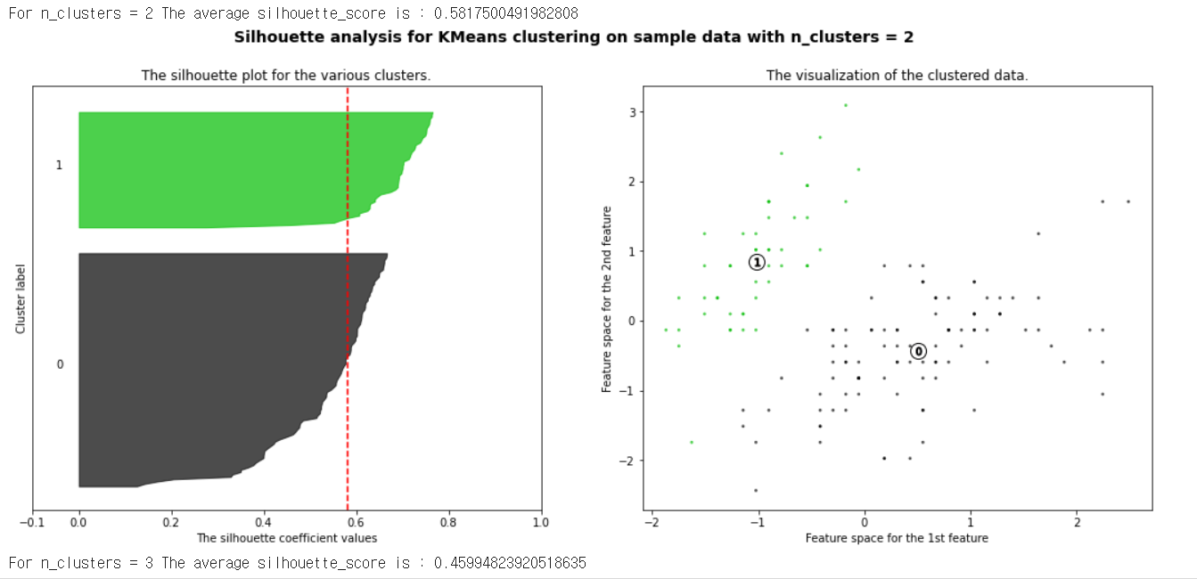
1번의 경우 모든 값이 평균(중간값)넘어 매우 이상적, 2번은 반정도만 넘어감. 스코어가 높을 수록 좋다