텍스트 마이닝
텍스트 마이닝을 군집화하여 감성분류 또한 할 수 있다.
텍스트를 계산 가능한 데이터로 처리하는 방법
- BoW(Bag of Words) : 가장 기본적인 방법, 각 형태소의 개수를 counting
- DTM(Document-Term Matrix) : 단어의 수
중요도 평가 방법
TF-IDF(Term Frequency-Inverse Document Frequency) : 단어의 중요도 계산
TF : 특정 문서에서 특정 단어의 등장 횟수
DF : 특정 단어가 등장한 문서의 수
IDF : DF와 반빕례 값을 가지는 수식
TF-IDF : TF, IDF를 곱한 값 -> 특정 문장에서 특출나게 나타나는 단어
문서에서 반복적으로 계속 나타나면 특정 문장에서는 그렇게 중요한 값이 아니며 틀정 문장에서만 자주 나타나는 단어가 문장의 핵심이라는 가설
예습
data : The Bourne Supremacy의 영화 script
Feature Description
page_no : 데이터가 위치한 pdf 페이지 정보
scene_title : 씬 제목
text : 씬에 해당하는 지문/대본 텍스트 정보
%matplotlib inline

import pandas as pd
import numpy as np
import matplotlib.pyplot as plt
import seaborn as sns

import warnings
warnings.filterwarnings("ignore")
df = pd.read_csv("https://raw.githubusercontent.com/yoonkt200/FastCampusDataset/master/bourne_scenario.csv")
데이터셋 기본 정보 확인
df.shape
df.isnull().sum()
df.info()
len(df['text'].values.sum())
데이터셋 전처리
정규표현식 적용
import re

def apply_regular_expression(text):
    text = text.lower() #소문자로 변환
    english = re.compile('[^ a-z]') #띄어쓰기를 포함한 알파벳으로 시작
    result = english.sub('', text) #
    result = re.sub(' +', ' ', result) # 공백 문자가 여러개 일때 하나로 바꾼다
    return result

df['processed_text'] = df['text'].apply(lambda x: apply_regular_expression(x)) # 전체 df에 함수 적용
df.head()
말뭉치(코퍼스) 생성
# make corpus
corpus = df['processed_text'].tolist()
corpus
BoW 생성
from sklearn.feature_extraction.text import CountVectorizer

# filter stop words
vect = CountVectorizer(tokenizer=None, stop_words="english", analyzer='word').fit(corpus) #token: 단어 문장단위로 어떻게 나눌지, stop_word:불용어, analyzer: 분석 단위
bow_vect = vect.fit_transform(corpus)
word_list = vect.get_feature_names() # 어떤 단어들이 들어가있는지 확인
count_list = bow_vect.toarray().sum(axis=0) # 인덱스순으로 몇개의 단어가 있는지
word_count_dict = dict(zip(word_list, count_list)) # word, count를 key value로 묶는 것

import operator

sorted(word_count_dict.items(), key=operator.itemgetter(1), reverse=True) # 빈도수가 높은 수로 정렬
단어 분포 검색
plt.hist(list(word_count_dict.values()), bins=150)
plt.show()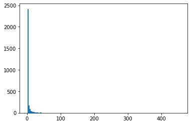
텍스트 마이닝
워드 클라우드 시각화 pytagcloud를 사용
!pip install pytagcloud pygame simplejsonfrom collections import Counter
import random
import pytagcloud
import webbrowser
ranked_tags = Counter(word_count_dict).most_common(25)
taglist = pytagcloud.make_tags(sorted(word_count_dict.items(), key=operator.itemgetter(1), reverse=True)[:40], maxsize=60)
pytagcloud.create_tag_image(taglist, 'wordcloud_example.jpg',
rectangular=False)
from IPython.display import Image
Image(filename='wordcloud_example.jpg')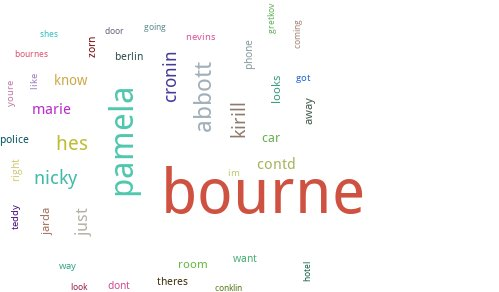
장면별 붕요단어 시각화
TF-IDF
from sklearn.feature_extraction.text import TfidfTransformer

tfidf_vectorizer = TfidfTransformer()
tf_idf_vect = tfidf_vectorizer.fit_transform(bow_vect)
print(tf_idf_vect.shape) #(320, 2850)
print(tf_idf_vect[0]) # 0번째 장의 단어들의 TF-IDF값
print(tf_idf_vect[0].toarray().shape)
print(tf_idf_vect[0].toarray())
단어 맵핑
invert_index_vectorizer = {v: k for k, v in vect.vocabulary_.items()} #아까 만들었던 단어들의 idex 모음
print(str(invert_index_vectorizer)[:100]+'..')
중요단어 추출
np.argsort(tf_idf_vect[0].toarray())[0][-3:] # 0장에서 값이 높은 top 3
np.argsort(tf_idf_vect.toarray())[:, -3:] # 각 장에서 top3
top_3_word = np.argsort(tf_idf_vect.toarray())[:, -3:]
df['important_word_indexes'] = pd.Series(top_3_word.tolist())
df.head()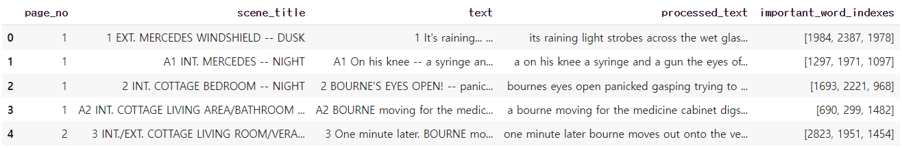
index를 word로 바꿔주면 됨
def convert_to_word(x):
    word_list = []
    for word in x:
        word_list.append(invert_index_vectorizer[word])
    return word_list

df['important_words'] = df['important_word_indexes'].apply(lambda x: convert_to_word(x))
df.head()
각 씬에대한 분위기를 유추할 수 있음
감성분류
순서
데이터 전처리
이진/다중 분류
그/부정 키워드 분석
리뷰의 댓글과 별점 데이터를 통해 모델을 제작
데이터셋 트립 어드바이저 제주도 호텔
Feature Description
rating : 이용자 리뷰의 평가 점수
text : 이용자 리뷰 평가 내용
%matplotlib inline

import pandas as pd
import numpy as np
import matplotlib.pyplot as plt
import seaborn as sns

import warnings
warnings.filterwarnings("ignore")
df = pd.read_csv("https://raw.githubusercontent.com/yoonkt200/FastCampusDataset/master/tripadviser_review.csv")
데이터 셋 파악
df.shape
df.isnull().sum()
df.info()
len(df['text'].values.sum())
전처리
# konlpy 0.5.2의 JVM 버그로 인해, 0.5.1 버전으로 install
!pip install konlpy==0.5.1 jpype1 Jpype1-py3
import re
def apply_regular_expression(text):
hangul = re.compile('[^ ㄱ-ㅣ가-힣]') # 한글의 정규표현식 특수문자 제거
result = hangul.sub('', text)
return result
apply_regular_expression(df['text'][0])'여행에 집중할수 있게 편안한 휴식을 제공하는 호텔이었습니다 위치선정 또한 적당한 편이었고 청소나 청결상태도 좋았습니다'
명사 형태소 분석
from konlpy.tag import Okt # 명사 형태소 분석 함수
from collections import Counter

nouns_tagger = Okt()
nouns = nouns_tagger.nouns(apply_regular_expression(df['text'][0])) #0번째 명사 형태소 추출
nouns = nouns_tagger.nouns(apply_regular_expression("".join(df['text'].tolist()))) # 전체 명사 형태소 추출
빈도수 확인
counter = Counter(nouns)
counter.most_common(10)
[('호텔', 803),
('수', 498),
('것', 436),
('방', 330),
('위치', 328),
('우리', 327),
('곳', 320),
('공항', 307),
('직원', 267),
('매우', 264)]
한글자 명사 제거 (필요없는 단어 제거)
available_counter = Counter({x : counter[x] for x in counter if len(x) > 1})
available_counter.most_common(10)
[('호텔', 803),
('위치', 328),
('우리', 327),
('공항', 307),
('직원', 267),
('매우', 264),
('가격', 245),
('객실', 244),
('시설', 215),
('제주', 192)]
매우 같은 불용어는 제거해야함
불용어 사전 제작
# source - https://www.ranks.nl/stopwords/korean
stopwords = pd.read_csv("https://raw.githubusercontent.com/yoonkt200/FastCampusDataset/master/korean_stopwords.txt").values.tolist()
print(stopwords[:10])
불용어 추가
jeju_hotel_stopwords = ['제주', '제주도', '호텔', '리뷰', '숙소', '여행', '트립']
for word in jeju_hotel_stopwords:
    stopwords.append(word)
BoW 생성
from sklearn.feature_extraction.text import CountVectorizer

def text_cleaning(text):
   hangul = re.compile('[^ ㄱ-ㅣ가-힣]') #정규표현식
   result = hangul.sub('', text)
   tagger = Okt()
   nouns = nouns_tagger.nouns(result)
   nouns = [x for x in nouns if len(x) > 1]
   nouns = [x for x in nouns if x not in stopwords] # 불용어 제거
   return nouns

vect = CountVectorizer(tokenizer = lambda x: text_cleaning(x))
bow_vect = vect.fit_transform(df['text'].tolist())
word_list = vect.get_feature_names() #단어 리스트
count_list = bow_vect.toarray().sum(axis=0) # 개수 리스트
딕 제작
word_count_dict = dict(zip(word_list, count_list))
word_count_dict
TF-IDF 변환
from sklearn.feature_extraction.text import TfidfTransformer

tfidf_vectorizer = TfidfTransformer()
tf_idf_vect = tfidf_vectorizer.fit_transform(bow_vect)
print(tf_idf_vect.shape)
print(tf_idf_vect[0])
단어 맵핑
invert_index_vectorizer = {v: k for k, v in vect.vocabulary_.items()} #맵핑 함수
print(str(invert_index_vectorizer)[:100]+'..')
Logistic Regression 분류
rating data를 이진으로 분류(3이하는 부정으로 가정)
def rating_to_label(rating):
    if rating > 3:
        return 1
    else:
        return 0

df['y'] = df['rating'].apply(lambda x: rating_to_label(x))
df.y.value_counts()
1 726
0 275
데이터 셋 분리
from sklearn.model_selection import train_test_split

y = df['y']
x_train, x_test, y_train, y_test = train_test_split(tf_idf_vect, y, test_size=0.30)
모델 학습
from sklearn.linear_model import LogisticRegression
from sklearn.metrics import accuracy_score, precision_score, recall_score, f1_score

# Train LR model
lr = LogisticRegression(random_state=0)
lr.fit(x_train, y_train)

# classifiacation predict
y_pred = lr.predict(x_test)
분류 결과 평가
# classification result for test dataset
print("accuracy: %.2f" % accuracy_score(y_test, y_pred))
print("Precision : %.3f" % precision_score(y_test, y_pred))
print("Recall : %.3f" % recall_score(y_test, y_pred))
print("F1 : %.3f" % f1_score(y_test, y_pred))
confusion matrix
from sklearn.metrics import confusion_matrix

# print confusion matrix
confmat = confusion_matrix(y_true=y_test, y_pred=y_pred)
print(confmat)
3 84
0 214
84쪽에 문제가 있음 편향된 예측을 하고 있음
샘플링 재조정
positive_random_idx = df[df['y']==1].sample(275, random_state=33).index.tolist()
negative_random_idx = df[df['y']==0].sample(275, random_state=33).index.tolist()
재학습 및 재평가
random_idx = positive_random_idx + negative_random_idx
X = tf_idf_vect[random_idx]
y = df['y'][random_idx]
x_train, x_test, y_train, y_test = train_test_split(X, y, test_size=0.25, random_state=33)

lr = LogisticRegression(random_state=0)
lr.fit(x_train, y_train)
y_pred = lr.predict(x_test)

print("accuracy: %.2f" % accuracy_score(y_test, y_pred))
print("Precision : %.3f" % precision_score(y_test, y_pred))
print("Recall : %.3f" % recall_score(y_test, y_pred))
print("F1 : %.3f" % f1_score(y_test, y_pred))

confmat = confusion_matrix(y_true=y_test, y_pred=y_pred)
print(confmat)
[[53 26
[12 47]]
대각선 값이 높은 것이 합리적
이를 토대로 긍정 및 부정 키워드 분석
Logistic Regression 모델의 coef 분석
# print logistic regression's coef
plt.rcParams['figure.figsize'] = [10, 8]
plt.bar(range(len(lr.coef_[0])), lr.coef_[0])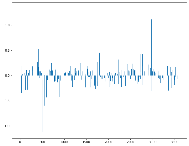
상위 하위 top 5 키워드 추출
print(sorted(((value, index) for index, value in enumerate(lr.coef_[0])), reverse=True)[:5])
print(sorted(((value, index) for index, value in enumerate(lr.coef_[0])), reverse=True)[-5:])
긍정, 부정순으로 정렬
coef_pos_index = sorted(((value, index) for index, value in enumerate(lr.coef_[0])), reverse=True)
coef_neg_index = sorted(((value, index) for index, value in enumerate(lr.coef_[0])), reverse=False)
coef_pos_index
맵핑
invert_index_vectorizer = {v: k for k, v in vect.vocabulary_.items()}긍정 키워드
for coef in coef_pos_index[:15]:
    print(invert_index_vectorizer[coef[1]], coef[0])
이용 1.3321308087111168
추천 1.1098677278465363
버스 1.029120247844704
최고 0.9474432432978868
가성 0.9049132254229898
근처 0.8631251640260484
조식 0.8624237330200107
다음 0.7848182816732695
위치 0.732990219026413
공간 0.716865493140725
시설 0.7161355390234533
맛집 0.7134163462461057
거리 0.7044600617626677
분위기 0.6869152801231841
바다 0.6556108465327279
부정 키워드
for coef in coef_neg_index[:15]:
    print(invert_index_vectorizer[coef[1]], coef[0])
냄새 -1.124500886987929
별로 -0.9632209931825515
아무 -0.6811855513119685
화장실 -0.6683241824194205
그냥 -0.6491883332225628
모기 -0.6302873381425533
수건 -0.6243491941007028
느낌 -0.5975494080979522
모텔 -0.5971174361320487
다른 -0.5966138818945081
최악 -0.593317479621261
음식 -0.5443424935120069
주위 -0.5321043465183405
진짜 -0.5254380815734122
목욕 -0.5087212885846032