학습할 내용

1. EDA(탐색적 데이터 분석)
2. Binary Classification - Logistic Regression
3. Clustering Classification - K-Means

활용한 데이터 셋 - 포켓본 데이터 셋

df = pd.read_csv("https://raw.githubusercontent.com/yoonkt200/FastCampusDataset/master/Pokemon.csv")

Feature Description
Name : 포켓몬 이름
Type 1 : 포켓몬 타입 1
Type 2 : 포켓몬 타입 2
Total : 포켓몬 총 능력치 (Sum of Attack, Sp. Atk, Defense, Sp. Def, Speed and HP)
HP : 포켓몬 HP 능력치
Attack : 포켓몬 Attack 능력치
Defense : 포켓몬 Defense 능력치
Sp. Atk : 포켓몬 Sp. Atk 능력치
Sp. Def : 포켓몬 Sp. Def 능력치
Speed : 포켓몬 Speed 능력치
Generation : 포켓몬 세대
Legendary : 전설의 포켓몬 여부

1. EDA(탐색적 데이터 분석)

기본적인 정보 탐색

df.shape
df.isnull().sum()
df.info()

개별 feature 탐색

df['Legendary'].value_counts() 
df['Generation'].value_counts().sort_index().plot() #index 별로 정리해서 plot
df['Generation'].value_counts().sort_index().hist() # hist로 plot 이건 오류가 남
df['Generation'].value_counts().sort_index().plot.barh() 로 보는게 제일 좋을 듯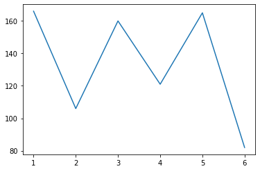 

홀수 세대의 포켓몬이 전반적으로 많은 것을 알 수 있음

타입의 개수 확인

len(df['Type 1'].unique())
len(df['Type 2'].unique())
len(df[df['Type 2'].notnull()]['Type 1'].unique())

변수들 분포 탐색

fig = plt.figure(figsize = (12, 12))
ax = fig.gca()
sns.boxplot(data=df[['HP', 'Attack', 'Defense', 'Sp. Atk', 'Sp. Def', 'Speed']], ax=ax)
plt.show()

#legenary만 탐색
fig = plt.figure(figsize = (12, 12))
ax = fig.gca()
sns.boxplot(data=df[df['Legendary']==1][['HP', 'Attack', 'Defense', 'Sp. Atk', 'Sp. Def', 'Speed']], ax=ax)
plt.show()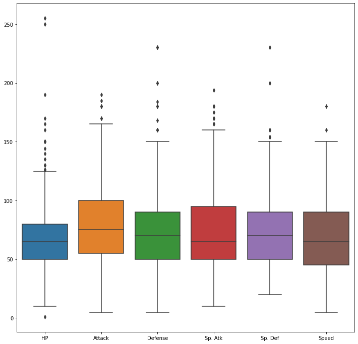

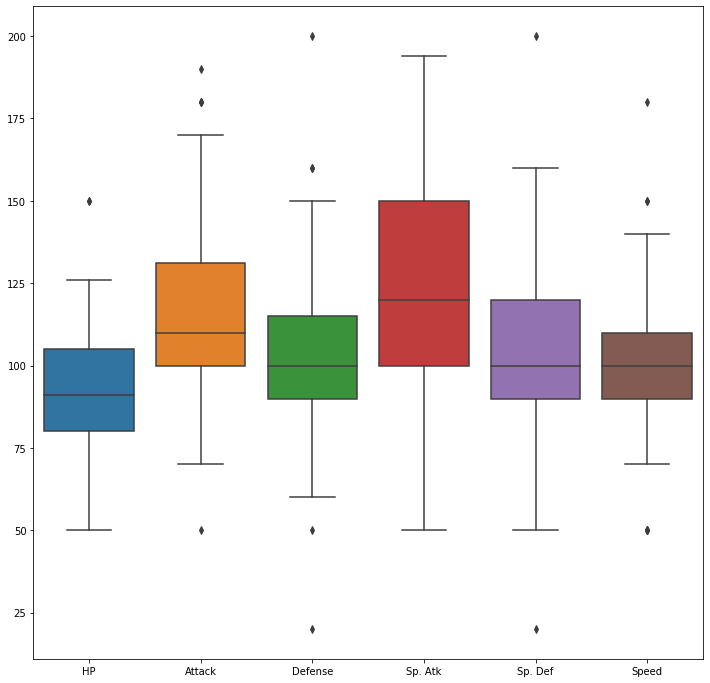
레전더리가 전반적으로 평균 수치가 전체 데이터에 비해 높게 형성되어 있는 것을 알 수 있다. hp 상승률이 다른 feature에 비해 낮다는 것을 알 수 있음

전체 능력치의 합

df['Total'].hist(bins=50)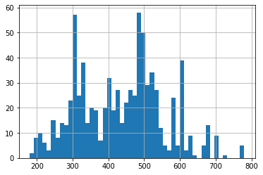

전체 스탯의 합이 600 이상인 포켓몬이 레전더리일 가능성이 높음

type feature에 따른 legendary 탐색

df['Type 1'].value_counts(sort=False).sort_index().plot.bar()
df[df['Legendary']==1]['Type 1'].value_counts(sort=False).sort_index().plot.barh()
df['Type 2'].value_counts(sort=False).sort_index().plot.barh()
df[df['Legendary']==1]['Type 2'].value_counts(sort=False).sort_index().plot.barh()

generation에 따른 legendary탐색

df['Generation'].value_counts().sort_index().plot.bar()
groups = df[df['Legendary']==1].groupby('Generation').size()
groups.plot.bar()

타입에 따른 스탯 차이

fig = plt.figure(figsize = (12, 12))
ax = fig.gca()
sns.boxplot(x = "Type 1", y = "Total", data=df, ax=ax)
plt.show()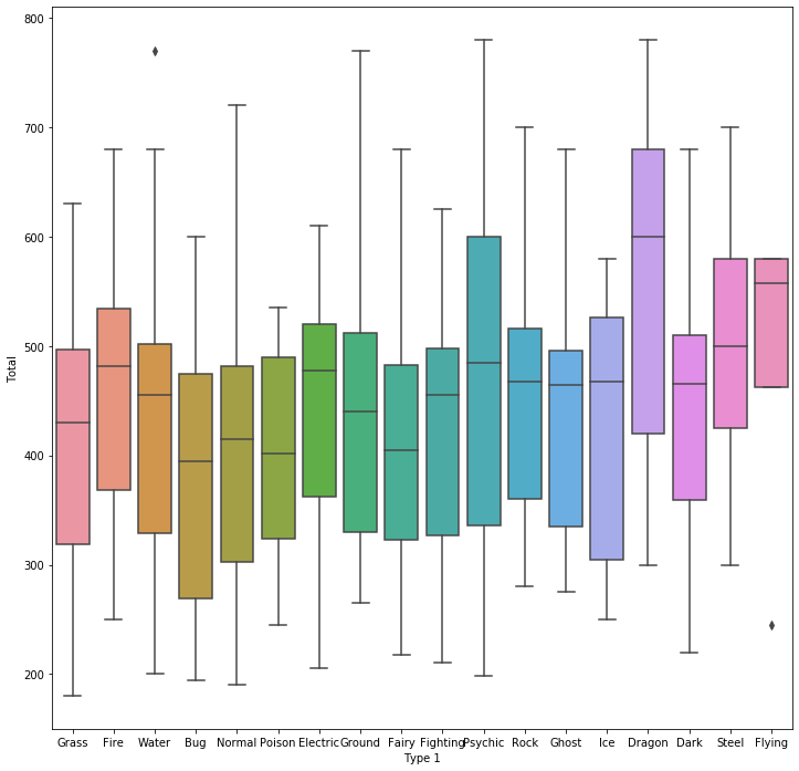

dragon, steel, flying 같은 type의 포켓몬이 전반적으로 스탯이 높다

2. Binary Classification - Logistic Regression

분류 분석의 종류

군집의 경우에는 class가 정해져 있는지 않는 비지도 학습임, 물론 class가 정해져 있는 model도 있기는 함

logistic function

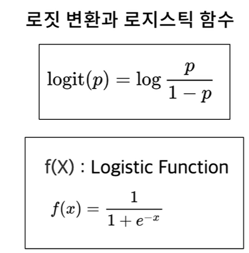
x가 음와 양에 따라 확률이 0과 1로구분시켜 주는 논리 함수

회귀분석에 사용되는 데이터 전처리

1. 원-핫 인코딩 : 카테고리형 범주형 데이터를 숫자로 표현하되 불필요한 상관관계를 만들지 않기 위해 더미데이터를 추가하는 전처리
   더 나아가 중복되는 클래스가 있는 경우 멀티 레이블 인코딩으로 해결

모델 평가 방법

1. Confusion Matrix
   
2. f1 score
3. AUC(Area Under Curve)

예제

전처리

df['Legendary'] = df['Legendary'].astype(int)
df['Generation'] = df['Generation'].astype(str)
preprocessed_df = df[['Type 1', 'Type 2', 'Total', 'HP', 'Attack', 
                      'Defense', 'Sp. Atk', 'Sp. Def', 'Speed', 'Generation', 'Legendary']]
preprocessed_df.head()

각 포켓몬은 타입을 두가지를 가지고 있기 때문에 multi label encoding이 필요

# pokemon type list 생성
def make_list(x1, x2):
    type_list = []
    type_list.append(x1)
    if x2 is not np.nan:
        type_list.append(x2)
    return type_list

preprocessed_df['Type'] = preprocessed_df.apply(lambda x: make_list(x['Type 1'], x['Type 2']), axis=1)
preprocessed_df.head()

del preprocessed_df['Type 1']
del preprocessed_df['Type 2']
preprocessed_df.head()

#multilabel binary encode
from sklearn.preprocessing import MultiLabelBinarizer
mlb = MultiLabelBinarizer()
preprocessed_df = preprocessed_df.join(pd.DataFrame(mlb.fit_transform(preprocessed_df.pop('Type')),
                                                    columns=mlb.classes_))

타입에 대한 전처리가 완료

이후 generation에 대한 one-hot encode

preprocessed_df = pd.get_dummies(preprocessed_df)
preprocessed_df.head()

feature standardization

from sklearn.preprocessing import StandardScaler

# feature standardization
scaler = StandardScaler()
scale_columns = ['Total', 'HP', 'Attack', 'Defense', 'Sp. Atk', 'Sp. Def', 'Speed']
preprocessed_df[scale_columns] = scaler.fit_transform(preprocessed_df[scale_columns])
preprocessed_df.head()

dataset 분리

from sklearn.model_selection import train_test_split

# dataset split to train/test
X = preprocessed_df.loc[:, preprocessed_df.columns != 'Legendary']
y = preprocessed_df['Legendary']
x_train, x_test, y_train, y_test = train_test_split(X, y, test_size=0.25, random_state=33)

logistic regression training

from sklearn.linear_model import LogisticRegression
from sklearn.metrics import accuracy_score, precision_score, recall_score, f1_score
# Train LR model
lr = LogisticRegression(random_state=0)
lr.fit(x_train, y_train)

# classifiacation predict
y_pred = lr.predict(x_test)

모델 평가

# classification result for test dataset
print("accuracy: %.2f" % accuracy_score(y_test, y_pred))
print("Precision : %.3f" % precision_score(y_test, y_pred))
print("Recall : %.3f" % recall_score(y_test, y_pred))
print("F1 : %.3f" % f1_score(y_test, y_pred))

#confusion matrix
from sklearn.metrics import confusion_matrix

# print confusion matrix
confmat = confusion_matrix(y_true=y_test, y_pred=y_pred)
print(confmat)

183 5
4 8
클래스의 분균형이 존재해서 정확도가 높게 나오는 것

target feature인 legendary를 분하기 위해서는 legendary에 대한 정보가 우선시 되어야함
데이터 sampling (legendary에서 65개 아닌것에서 65개 뽑아서 새로 샘플링)

positive_random_idx = preprocessed_df[preprocessed_df['Legendary']==1].sample(65, random_state=33).index.tolist()
negative_random_idx = preprocessed_df[preprocessed_df['Legendary']==0].sample(65, random_state=33).index.tolist()
positive_random_idx # 뽑은것 확인

새로 데이터 셋 분류 및 재 학습 후 평가

# dataset split to train/test
random_idx = positive_random_idx + negative_random_idx
X = preprocessed_df.loc[random_idx, preprocessed_df.columns != 'Legendary']
y = preprocessed_df['Legendary'][random_idx]
x_train, x_test, y_train, y_test = train_test_split(X, y, test_size=0.25, random_state=33)

# Train LR model
lr = LogisticRegression(random_state=0)
lr.fit(x_train, y_train)

# classifiacation predict
y_pred = lr.predict(x_test)

# classification result for test dataset
print("accuracy: %.2f" % accuracy_score(y_test, y_pred))
print("Precision : %.3f" % precision_score(y_test, y_pred))
print("Recall : %.3f" % recall_score(y_test, y_pred))
print("F1 : %.3f" % f1_score(y_test, y_pred))
# f1스코어가 증가한 것을 알 수 있음

# print confusion matrix
confmat = confusion_matrix(y_true=y_test, y_pred=y_pred)
print(confmat)

20 1
0 12

3. Clustering Classification - K-Means

Kmeans 군집 분류 : 주어진 데이터를 k개의 클러스터로 묶는 방식, 거리 차이의 분산을 최소화하는 방식으로 동작

처음에 사용자가 정한 k개의 임의의 점을 골라 clustering을 하고 그 값들의 평균을 내어 새로 중심값을 설정 이를 반복하여 clustering을 진행

차원의 커질수록 계산이 복잡해지는 차원의 저주 3~4차원의 경우에는 효율 적이지 않음 그렇기 때문에 차원 축소를 하는 것이 좋음

해석 방법
1. elbow method(엘보우 메소드) : 차원축소를 하였을 때 clustering을 평가, k값을 여러개로 바꾸어 보면서 최적을 k를 찾음. 특정 지점에서 값이 어느정도 수렴하는데 그 이상으로 k을 늘려도 큰 의미가 없다는 것을 알려줌. 그래프가 사람의 팔과 닮아서 elbow라는 표현을 씀
2. silhouette method(실루엣)

예제

능력치에 따른 포켓몬 분집 분류

kmeans 군집분류 2차원 attck, depense

from sklearn.cluster import KMeans

# K-means train & Elbow method
X = preprocessed_df[['Attack', 'Defense']]

k_list = []
cost_list = []
for k in range (1, 6):
    kmeans = KMeans(n_clusters=k).fit(X)
    interia = kmeans.inertia_
    print ("k:", k, "| cost:", interia)
    k_list.append(k)
    cost_list.append(interia)
    
plt.plot(k_list, cost_list)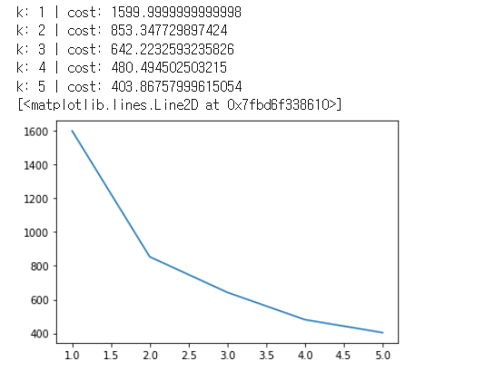

4개 정도가 적당해 보임

예측

kmeans = KMeans(n_clusters=4).fit(X)
cluster_num = kmeans.predict(X)
cluster = pd.Series(cluster_num)
preprocessed_df['cluster_num'] = cluster.values
preprocessed_df.head()
print(preprocessed_df['cluster_num'].value_counts()) # clustering이 어느정도 비율로 나누어 졌는지

데이터 시각화

# Visualization
plt.scatter(preprocessed_df[preprocessed_df['cluster_num'] == 0]['Attack'], 
            preprocessed_df[preprocessed_df['cluster_num'] == 0]['Defense'], 
            s = 50, c = 'red', label = 'Pokemon Group 1')
plt.scatter(preprocessed_df[preprocessed_df['cluster_num'] == 1]['Attack'], 
            preprocessed_df[preprocessed_df['cluster_num'] == 1]['Defense'], 
            s = 50, c = 'green', label = 'Pokemon Group 2')
plt.scatter(preprocessed_df[preprocessed_df['cluster_num'] == 2]['Attack'], 
            preprocessed_df[preprocessed_df['cluster_num'] == 2]['Defense'], 
            s = 50, c = 'blue', label = 'Pokemon Group 3')
plt.scatter(preprocessed_df[preprocessed_df['cluster_num'] == 3]['Attack'], 
            preprocessed_df[preprocessed_df['cluster_num'] == 3]['Defense'], 
            s = 50, c = 'yellow', label = 'Pokemon Group 4')
plt.title('Pokemon Cluster by Attack, Defense')
plt.xlabel('Attack')
plt.ylabel('Defense')
plt.legend()
plt.show()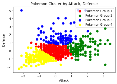

kmeans 군집분류 다차원

from sklearn.cluster import KMeans

# K-means train & Elbow method
X = preprocessed_df[['HP', 'Attack', 'Defense', 'Sp. Atk', 'Sp. Def', 'Speed']]

k_list = []
cost_list = []
for k in range (1, 15):
    kmeans = KMeans(n_clusters=k).fit(X)
    interia = kmeans.inertia_
    print ("k:", k, "| cost:", interia)
    k_list.append(k)
    cost_list.append(interia)
    
plt.plot(k_list, cost_list)

5~6정도에 팔꿈치 존재

모델 학습

# selected by elbow method (5)
kmeans = KMeans(n_clusters=5).fit(X)
cluster_num = kmeans.predict(X)
cluster = pd.Series(cluster_num)
preprocessed_df['cluster_num'] = cluster.values
preprocessed_df.head()

군집별 특성 시각화 : 다차원이기 때문에 EDA로 데이터의 특성을 확인해야한다.

fig = plt.figure(figsize = (12, 12))
ax = fig.gca()
sns.boxplot(x = "cluster_num", y = "HP", data=preprocessed_df, ax=ax)
plt.show()

1, 3이 전반적으로 hp가 높다. 0의 경우에는 모든 군집중에 가장 hp가 낮다

fig = plt.figure(figsize = (12, 12))
ax = fig.gca()
sns.boxplot(x = "cluster_num", y = "Attack", data=preprocessed_df, ax=ax)
plt.show()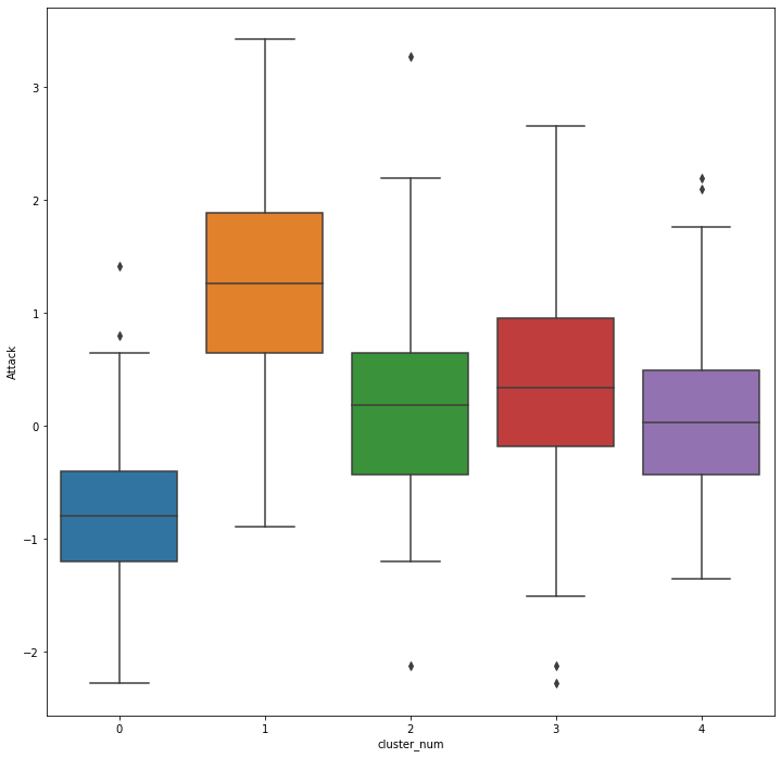

0번은 공격력도 낮고 1번 군집은 공격력이 매우 높음

fig = plt.figure(figsize = (12, 12))
ax = fig.gca()
sns.boxplot(x = "cluster_num", y = "Defense", data=preprocessed_df, ax=ax)
plt.show()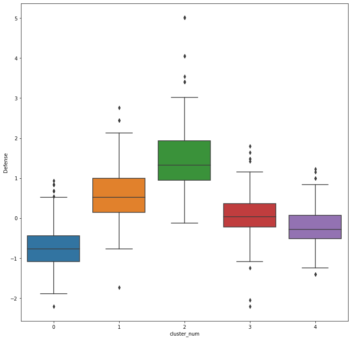

0번은 depense도 낮은 것으로 보아 0번 포켓몬은 가장 약한 포켓몬의 집단인 것을 알 수 있다.
2번의 경우 방어력이 압도적으로 높은데 방어 지향 포켓몬인 것을 알 수 있음

fig = plt.figure(figsize = (12, 12))
ax = fig.gca()
sns.boxplot(x = "cluster_num", y = "Sp. Atk", data=preprocessed_df, ax=ax)
plt.show()

sp.attak이 강력한 집단은 1번 이다.

fig = plt.figure(figsize = (12, 12))
ax = fig.gca()
sns.boxplot(x = "cluster_num", y = "Sp. Def", data=preprocessed_df, ax=ax)
plt.show()

spdef이 1번이 높다.
전반적으로 1번이 모든 스탯이 높은것으로 보아 legendary일 확률이 높다는 것을 알 수 있다.

fig = plt.figure(figsize = (12, 12))
ax = fig.gca()
sns.boxplot(x = "cluster_num", y = "Speed", data=preprocessed_df, ax=ax)
plt.show()

이 데이터를 통해 4번이 스피드 형 타입인 것을 알 수 있다.

또한 3번의 경우에는 밸런스 형일 가능 성이 높다는 것을 알 수 있다.