이번에도 텐서플로우의 기본 데이터셋으로 딥러닝을 연습해보려고 한다.

---

import 코드

import numpy as np
import pandas as pd
import tensorflow as tf

import matplotlib.pyplot as plt
import seaborn as sns
%matplotlib inline

matplotilb.pyplot와 seaborn까지 import해주어 그림으로도 살펴볼 예정이다.

데이터셋

TensorFlow에서 제공하는 MNIST 예제를 다루어 볼 것이다.

• 데이터 shape, dtype 확인하기

(train_x, train_y), (test_x, test_y) = tf.keras.datasets.mnist.load_data()

print(train_x.shape)
print(test_x.shape)

(60000, 28, 28)
(10000, 28, 28)

다음과 같은 x에 대한 shape 모양을 확인할 수 있다.

print(train_y.shape)
print(test_y.shape)

(60000,)
(10000,)

y에 대한 shape도 살펴보자

• dtype

print(train_x.dtype)
print(test_x.dtype)

print(train_y.dtype)
print(test_y.dtype)

uint8
uint8
uint8
uint8

데이터 하나만 뽑아보기

image = train_x[77]
image.shape

(28, 28)

시각화

plt.imshow(image, 'gray')
plt.show()

훈련용 데이터셋에는 각 숫자의 그림이 몇개씩 들어가 있을까?

y_unique, y_counts = np.unique(train_y, return_counts=True)
print(y_unique, y_counts)

[0 1 2 3 4 5 6 7 8 9][5923 6742 5958 6131 5842 5421 5918 6265 5851 5949]
물음에 대한 답을 간단하게 찾을 수 있다.
그러면 시각화를 해서 보기 쉽도록 만들어보자

df_view = pd.DataFrame(data={"count" : y_counts}, index=y_unique)
df_view

df_view.sort_values("count", ascending=False)

plt.bar(x=y_unique, height=y_counts, color="black")
plt.title("label distribution")
plt.show()

preprocessing

데이터 검증

• 데이터 중에 학습에 포함 되면 안되는 것이 있는가? ex> 개인정보가 들어있는 데이터, 테스트용 데이터에 들어있는것, 중복되는 데이터
• 학습 의도와 다른 데이터가 있는가? ex> 얼굴을 학습하는데 발 사진이 들어가있진 않은지(가끔은 의도하고 일부러 집어넣는 경우도 있음)
• 라벨이 잘못된 데이터가 있는가? ex> 7인데 1로 라벨링, 고양이 인데 강아지로 라벨링

def validate_pixel_scale(x):

    return 255 >= x.max() and 0 <= x.min()

validated_train_x = np.array([x for x in train_x if validate_pixel_scale(x)])

validated_train_y = np.array([y for x, y in zip(train_x, train_y) if validate_pixel_scale(x)])


print(validated_train_x.shape)
print(validated_train_y.shape)

(60000, 28, 28)
(60000,) 값을 얻을 수 있다.

전처리

• 입력하기 전에 모델링에 적합하게 처리!
• 대표적으로 Scaling, Resizing, label encoding 등이 있다.
• dtype, shape 항상 체크!!

scaling

def scale(x):
    """
    Make pixels within 0 ~ 1
    
    return 
        scaled image (dtype=float32)
    """
    return (x / 255.0).astype(np.float32)

# unit test
sample = scale(validated_train_x[777])
print(sample.max())

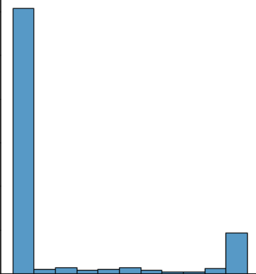
sns.displot(sample.reshape(-1), kde=False)
plt.show()

1.0

scaled_train_x = np.array([scale(x) for x in validated_train_x])

print(scaled_train_x.shape, scaled_train_x.dtype)

(60000, 28, 28) float32
shape를 확일할 수 있었다.

하나의 클래스로 만들어보기

class DataLoader():
    def __init__(self):
        # data load
        (self.train_x, self.train_y), \
            (self.test_x, self.test_y) = tf.keras.datasets.mnist.load_data()

    def validate_pixel_scale(self, x):

        return 255 >= x.max() and 0 <= x.min()

    def scale(self, x):
        """
        Make pixels within 0 ~ 1

        return 
            scaled image (dtype=float32)
        """
        return (x / 255.0).astype(np.float32)

    def preprocess_dataset(self, dataset):
        """
        feature 
            shape : (num_data, 28, 28)
        target 
            shape : (num_data,)

        return 
            feature 
                shape : (num_data, 28, 28)
            target 
                shape : (num_data,)
        """
        (feature, target) = dataset

        validated_x = np.array(
            [x for x in feature if self.validate_pixel_scale(x)])

        validated_y = np.array([y for x, y in zip(feature, target)
                                if self.validate_pixel_scale(x)])

        # scaling #
        scaled_x = np.array([self.scale(x) for x in validated_x])

        # flattening #
        flattend_x = scaled_x.reshape((scaled_x.shape[0], -1))

        # label encoding #
        ohe_y = np.array([tf.keras.utils.to_categorical(
            y, num_classes=10) for y in validated_y])
        
        return flattend_x, ohe_y

    def get_train_dataset(self):
        return self.preprocess_dataset((self.train_x, self.train_y))

    def get_test_dataset(self):
        return self.preprocess_dataset((self.test_x, self.test_y))

mnist_loader = DataLoader()

train_x, train_y = mnist_loader.get_train_dataset()
print(train_x.shape, train_x.dtype)
print(train_y.shape, train_y.dtype)

(60000, 784) float32
(60000, 10) float32

test_x, test_y = mnist_loader.get_test_dataset()
print(test_x.shape, test_x.dtype)
print(test_y.shape, test_y.dtype)

(10000, 784) float32
(10000, 10) float32

train과 test의 각 dtype과 shape를 확인할 수 있었다.

Modeling

1. 모델 정의
2. 학습 로직 - 비용함수, 학습파라미터 세팅
3. 학습

모델 정의

from tensorflow.keras.layers import Dense, Activation

model = tf.keras.Sequential()
model.add(Dense(15, input_dim=784))
model.add(Activation('sigmoid'))
model.add(Dense(10, input_dim=784))
model.add(Activation('softmax'))

model.summary()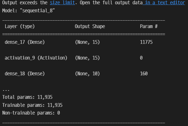

학습 로직

learning_rate = 0.03
opt = tf.keras.optimizers.SGD(learning_rate)
loss = tf.keras.losses.categorical_crossentropy

model.compile(optimizer=opt, loss=loss, metrics=["accuracy"])

학습 실행

batch_size = 128 # default == 32
epochs = 10

hist = model.fit(train_x,
                 train_y,
                 batch_size=batch_size,
                 epochs=epochs)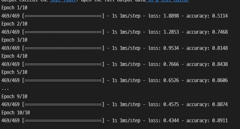

10개의 epochs가 돌아가는 것을 확인했다.

Evalution

• 학습 과정 추적
• Test / 모델 검증
• 후처리

학습 과정 추적

plt.figure(figsize=(10, 5))
plt.subplot(121)
plt.plot(hist.history['loss'])
plt.title("loss")
plt.ylabel("loss")
plt.subplot(122)
plt.plot(hist.history['accuracy'], 'b-')
plt.title("acc")
plt.ylabel("acc")
plt.tight_layout()
plt.show()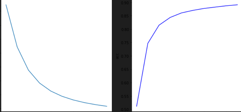

모델 검증

model.evaluate(test_x, test_y)

[0.4133513271808624, 0.8978999853134155]