CNN이란
이미지를 분석하기 위한 패턴을 찾는데 유용한 알고리즘이고
이미지를 직접 학습하고 패턴을 사용해 이미지를 분류한다.
구조
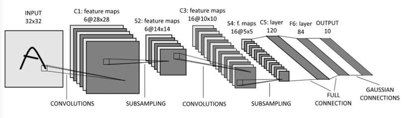
input – C1 – S2 – C3 – S4 – C5 – F6 - output
Flatten => 채널 차원 추가로 변경
(Convolution Layer는 주로 이미지데이터처리를 위해 사용되기 때문에, 컬러이미지는 (height, width, 3) 흑백은 (height, width, 1)로 사용한다.)
ex) (num_data, 28, 28) => (num_data, 28, 28, 1)
class DataLoader():
    def __init__(self):
        # data load
        (self.train_x, self.train_y), \
            (self.test_x, self.test_y) = tf.keras.datasets.mnist.load_data()

    def scale(self, x):

        return (x / 255.0).astype(np.float32)

    def preprocess_dataset(self, dataset):

        (feature, target) = dataset

        # scaling #
        scaled_x = np.array([self.scale(x) for x in feature])

        # Add channel axis #
        expanded_x = scaled_x[:, :, :, np.newaxis]

        # label encoding #
        ohe_y = np.array([tf.keras.utils.to_categorical(
            y, num_classes=10) for y in target])

        return expanded_x, ohe_y

    def get_train_dataset(self):
        return self.preprocess_dataset((self.train_x, self.train_y))

    def get_test_dataset(self):
        return self.preprocess_dataset((self.test_x, self.test_y))
mnist_loader = DataLoader()
train_x, train_y = mnist_loader.get_train_dataset()
print(train_x.shape, train_x.dtype)
print(train_y.shape, train_y.dtype)
test_x, test_y = mnist_loader.get_test_dataset()
print(test_x.shape, test_x.dtype)
print(test_y.shape, test_y.dtype)(60000, 28, 28, 1) float32
(60000, 10) float32
(10000, 28, 28, 1) float32
(10000, 10) float32
VGGNet에서 사용되는 Layer들
tf.keras.layers.Conv2Dtf.keras.layers.Activationtf.keras.layers.MaxPool2Dtf.keras.layers.Flattentf.keras.layers.Dense
Conv2D
- filters: layer에서 사용할 Filter(weights)의 갯수
- kernel_size: Filter(weights)의 사이즈
- strides: 몇 개의 pixel을 skip 하면서 훑어지나갈 것인지 (출력 피쳐맵의 사이즈에 영향을 줌)
- padding: zero padding을 만들 것인지. VALID는 Padding이 없고, SAME은 Padding이 있음 (출력 피쳐맵의 사이즈에 영향을 줌)
- activation: Activation Function을 지정
MaxPool2D
- pool_size: Pooling window 크기
- strides: 몇 개의 pixel을 skip 하면서 훑어지나갈 것인지
- padding: zero padding을 만들 것인지
Dense
- units : 노드 갯수
- activation : 활성화 함수
- use_bias : bias 를 사용 할 것인지
- kernel_initializer : 최초 가중치를 어떻게 세팅 할 것인지
- bias_initializer : 최초 bias를 어떻게 세팅 할 것인지
Layer들을 이용해 모델 만들기 - Sequencial 방식
from tensorflow.keras.layers import Conv2D, MaxPool2D, Flatten, Densemodel = tf.keras.Sequential()
# 최초의 레이어는 Input의 shape을 명시해준다. (이 때 배치 axis는 무시한다.)
model.add(Conv2D(32, kernel_size=3, padding='same', activation='relu', input_shape=(28, 28, 1)))
model.add(Conv2D(32, kernel_size=3, padding='same', activation='relu'))
model.add(MaxPool2D())
model.add(Conv2D(64, kernel_size=3, padding='same', activation='relu', input_shape=(28, 28, 1)))
model.add(Conv2D(64, kernel_size=3, padding='same', activation='relu'))
model.add(MaxPool2D())
model.add(Flatten())
model.add(Dense(128, activation="relu"))
model.add(Dense(64, activation="relu"))
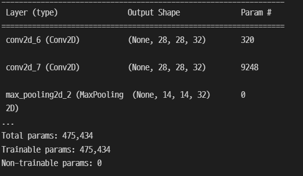
model.add(Dense(10, activation="softmax"))model.summary()를 봐보자..
이번에는 학습을 시킬 수 있도록 model 설정을 해야한당!
learning_rate = 0.03
opt = tf.keras.optimizers.Adam(learning_rate)
loss = tf.keras.losses.categorical_crossentropy

model.compile(optimizer=opt, loss=loss, metrics=["accuracy"])


hist = model.fit(train_x, train_y,
                 epochs=2, batch_size=128,
                 validation_data=(test_x, test_y))
plt.figure(figsize=(10, 5))
plt.subplot(221)
plt.plot(hist.history['loss'])
plt.title("loss")
plt.subplot(222)
plt.plot(hist.history['accuracy'], 'b-')
plt.title("acc")
plt.subplot(223)
plt.plot(hist.history['val_loss'])
plt.title("val_loss")
plt.subplot(224)
plt.plot(hist.history['val_accuracy'], 'b-')
plt.title("val_accuracy")
plt.tight_layout()
plt.show()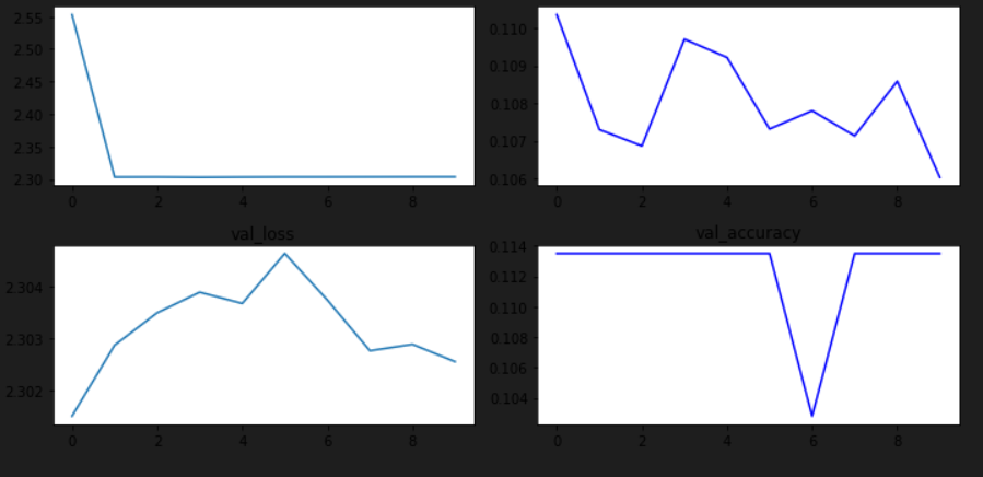

문과생 데이터사이언티스트되기 프로젝트