10. 결정트리

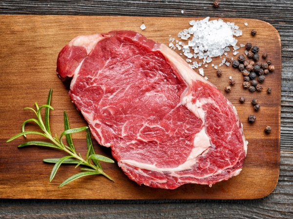
와인의 당도, 도수, 산도만으로 화이트/레드 와인을 나누어 볼것이다.

로지스틱 회귀 이용

우선 와인 정보를 받아보자

import pandas as pd
wine = pd.read_csv('https://bit.ly/wine_csv_data')

wine.info()
"""
 #   Column   Non-Null Count  Dtype  
---  ------   --------------  -----  
 0   alcohol  6497 non-null   float64
 1   sugar    6497 non-null   float64
 2   pH       6497 non-null   float64
 3   class    6497 non-null   float64
"""
print(wine.describe())
"""
dtypes: float64(4)
memory usage: 203.2 KB
           alcohol        sugar           pH        class
count  6497.000000  6497.000000  6497.000000  6497.000000
mean     10.491801     5.443235     3.218501     0.753886
std       1.192712     4.757804     0.160787     0.430779
min       8.000000     0.600000     2.720000     0.000000
25%       9.500000     1.800000     3.110000     1.000000
50%      10.300000     3.000000     3.210000     1.000000
75%      11.300000     8.100000     3.320000     1.000000
max      14.900000    65.800000     4.010000     1.000000
"""

data = wine[['alcohol','sugar','pH']].to_numpy()
target = wine['class'].to_numpy()

from sklearn.model_selection import train_test_split
train_input, test_input, train_target, test_target = \
    train_test_split(data,target,test_size=0.2,random_state=42)

위 info()와 describe() 메소드를 통하여 데이터의 정보를 확인 가능하다

from sklearn.preprocessing import StandardScaler
ss = StandardScaler()
ss.fit(train_input)
train_scaled = ss.transform(train_input) # 0.7808350971714451
test_scaled = ss.transform(test_input) # 0.7776923076923077
print(lr.coef_,lr.intercept_) 
# [[ 0.51270274  1.6733911  -0.68767781]] [1.81777902]

높은 점수는 아니지만, 어느정도 작동 가능한 모델이 완성되었다

모델 설명

이제 해당 모델을 고객 혹은 상급자에게 설명을 해보자

"도수값에 0.512..., 당도에 1.6733..., 산도에 -0.687... 값을 곱한 후 1.817... 을 더한 값이 0보다 크만 화이트, 작으면 레드와인...

설명에 있어 확실히 난해한 부분이 많다

결정 트리

결정 트리 모델은 이러한 상황에서 강점을 가진다
해당 모델이 어떤 식으로 동작하는지 이유를 설명하기 매우 쉽다

from sklearn.tree import DecisionTreeClassifier
dt = DecisionTreeClassifier()
dt.fit(train_scaled, train_target)
print_score(dt,"dt")
# 0.996921300750433
# 0.8592307692307692

과대적합이 조금 일어났지만, 어느정도 양호한 모델이 나왔다
이제 해당 모델은 그림으로 표현해보자

import matplotlib.pyplot as plt
from sklearn.tree import plot_tree
plt.figure(figsize=(10,7))
plot_tree(dt)
plt.show()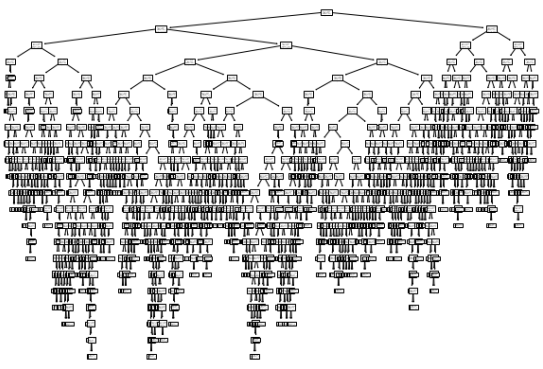

이런 복잡한 트리구조가 나오는데, 좀 더 그림을 간략화 시켜보자

plot_tree(dt, max_depth=1, filled=True, feature_names=['alcohol','sugar','pH'])

filled는 분류에 따른 색을, feature_names는 매개변수 이름을 지정 가능하다

gini 불순도

그림에서 보면 gini라는것이 존재한다
해당 데이터가 얼마나 잘 분할되어있는지 분류하는 지수이다
$(지니불순도) = 1-(음성 클래스 비율^2 + 양성 클래스 비율^2)$
부모와 자식 사이에서 불순도의 차이를 정보이득이라고 하며, gini가 낮을수록 더 이득임을 알 수 있다

가지치기

더 제대로 동작하는 트리를 만들기 위해, 가지치기를 할 필요가 있다
max_depth 값을 조정하여 가지치기를 해보자

from sklearn.tree import DecisionTreeClassifier
dt = DecisionTreeClassifier(max_depth=3, random_state=42)
dt.fit(train_scaled, train_target)
print_score(dt,"dt")
# 0.8454877814123533
# 0.8415384615384616

import matplotlib.pyplot as plt
from sklearn.tree import plot_tree
plt.figure(figsize=(20,15))
plot_tree(dt, filled=True, feature_names=['alcohol','sugar','pH'])
plt.show()

음수인 당도

그런데 트리를 보니가 당이 음수인 곳이 있다
해당 모델을 전처리 작업 후 훈련시켰기에 일어난 결과이다.
트리 알고리즘은 스케일에 따라 영향을 받지 않기에 이러한 전처리 작업이 필요없다

from sklearn.tree import DecisionTreeClassifier
dt = DecisionTreeClassifier(max_depth=3, random_state=42)
dt.fit(train_input, train_target)
print_score(dt,"dt")
# 0.8454877814123533
# 0.8415384615384616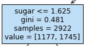

결과값도 같으며, 분류하는 트리 정보또한 직관적으로 작성되었다