Contrastive Embedding for Generalized Zero-Shot Learning 제5-2부

---

The effect of different embedding models (E-M) and different spaces in the hybrid GZSL framework.
하이브리드 GZSL 프레임워크에서 다양한 임베딩 모델(E-M)과 다른 공간의 효과.
All the methods here are combined with the feature generation model.
여기의 모든 방법은 기능 생성 모델과 결합됩니다.
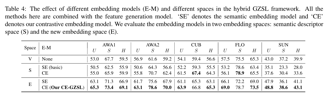
‘SE’ denotes the semantic embedding model and ‘CE’ denotes our contrastive embedding model. We evaluate the embedding models in two embedding spaces: semantic descriptor space (S) and the new embedding space (E).
'SE'는 시맨틱 임베딩 모델을 나타내고 'CE'는 대조 임베딩 모델을 나타냅니다. 의미 설명자 공간(S)과 새로운 임베딩 공간(E)의 두 가지 임베딩 공간에서 임베딩 모델을 평가합니다.

---

In Table 4, we investigate the effect of different spaces and different embedding models in the hybrid GZSL framework.
표 4에서 우리는 하이브리드 GZSL 프레임워크에서 다른 공간과 다른 임베딩 모델의 효과를 조사합니다.

We integrate the feature generation model with two different embedding models: semantic embedding (SE) (i.e. the ranking loss method) and our contrastive embedding (CE).
우리는 기능 생성 모델을 두 가지 다른 임베딩 모델, 즉 SE(Semantic Embedding)(즉, 순위 손실 방법)와 대조 임베딩(CE)과 통합합니다.

And we evaluate the semantic descriptor space (S) and the new embedding space (E), in which we conduct the final GZSL classification.
그리고 최종 GZSL 분류를 수행하는 의미 설명자 공간(S)과 새로운 임베딩 공간(E)을 평가합니다.

Firstly, we evaluate the same embedding model on different embedding spaces: the results of ‘SE’ on the new embedding space performs much better than ‘SE (basic)’ on the semantic space; and ‘CE (Our CE-GZSL)’ on the new embedding space also performs better than ‘CE’ on the semantic descriptor space.
첫째, 다른 임베딩 공간에서 동일한 임베딩 모델을 평가합니다. 그리고 새로운 임베딩 공간의 'CE(Our CE-GZSL)'도 시맨틱 디스크립터 공간의 'CE'보다 더 나은 성능을 보입니다.

---

This demonstrates that the new embedding space is much more effective than the original semantic space in our hybrid framework.
이것은 새로운 임베딩 공간이 하이브리드 프레임워크의 원래 의미 공간보다 훨씬 더 효과적이라는 것을 보여줍니다.

Afterward, we compare the results on the same embedding space but using different embedding models: ‘SE’ corresponds to the ranking loss form in Eq.3 and ‘CE’ corresponds to contrastive form in Eq.7.
afterward 그런다음
그런 다음 동일한 임베딩 공간에서 다른 임베딩 모델을 사용하여 결과를 비교합니다. 'SE'는 Eq.3의 순위 손실 형식에 해당하고 'CE'는 Eq.7의 대조 형식에 해당합니다.

Our proposed ‘CE’ can always outperform ‘SE’, no matter in the semantic descriptor space or in the new embedding space.
우리가 제안한 'CE'는 시맨틱 디스크립터 공간이나 새로운 임베딩 공간에서 항상 'SE'를 능가할 수 있습니다.

This illustrates that our contrastive embedding (CE) benefits from the instance-wise supervision which is neglected in the traditional semantic embedding (SE).
이것은 우리의 대조적 임베딩(CE)이 전통적인 의미론적 임베딩(SE)에서 무시되는 인스턴스별 감독의 이점을 보여줍니다.

---

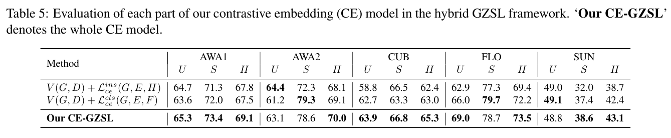
Evaluation of each part of our contrastive embedding (CE) model in the hybrid GZSL framework. ‘Our CE-GZSL’ denotes the whole CE model.
하이브리드 GZSL 프레임워크에서 대조 임베딩(CE) 모델의 각 부분에 대한 평가. 'Our CE-GZSL'은 전체 CE 모델을 나타냅니다.

---

Moreover, in Table 5, we respectively evaluate the instance-level supervision and the class-level supervision in our contrastive embedding model.
또한 표 5에서 대조 임베딩 모델에서 인스턴스 수준 감독과 클래스 수준 감독을 각각 평가합니다.

Concretely, to evaluate the instance-level supervision, we remove the classlevel supervision $\mathcal{L}_{ce}^{cls}(G, E, F)$ in Eq.9 and only optimize $V(G, D) + \mathcal L^{ins}_{ce} (G, E, H)$ to learn our contrastive embedding model.
구체적으로, 인스턴스 수준의 감독을 평가하기 위해 Eq.9에서 클래스 수준의 감독 $\mathcal{L}_{ce}^{cls}(G, E, F)$를 제거하고 $V(G, D) + \mathcal L^{ins}_{ce} (G, E, H)$만 최적화합니다. 대조적 임베딩 모델을 배우기 위해

In the same way, we evaluate the class-level supervision by optimizing $V(G, D) + \mathcal L^{cls}_{ce} (G, E, F)$.
in the same way 같은 방식으로
같은 방식으로 V(G, D) + L cls ce(G, E, F)를 최적화하여 클래스 수준의 감독을 평가합니다.

As shown in Table 5, when using either the instance-level CE or the class-level CE, our result is still competitive compared with the state-of-the-art GZSL methods.
<표 5>에서 보는 바와 같이 인스턴스 수준의 CE나 클래스 수준의 CE를 사용했을 때, 우리의 결과는 여전히 최신 GZSL 방식에 비해 경쟁력이 있다.

When considering both the instance-level supervision and the class-level supervisions, our method achieves the improvements on U and S, leading to the better H results.
인스턴스 수준의 감독과 클래스 수준의 감독을 모두 고려할 때 우리의 방법은 U와 S에 대한 개선을 달성하여 더 나은 H 결과로 이어집니다.

This means that our method benefits from the combination of the instance-level supervision and the class-level supervision.
이것은 우리의 방법이 인스턴스 수준 감독과 클래스 수준 감독의 조합으로부터 이점을 얻는다는 것을 의미합니다.

---

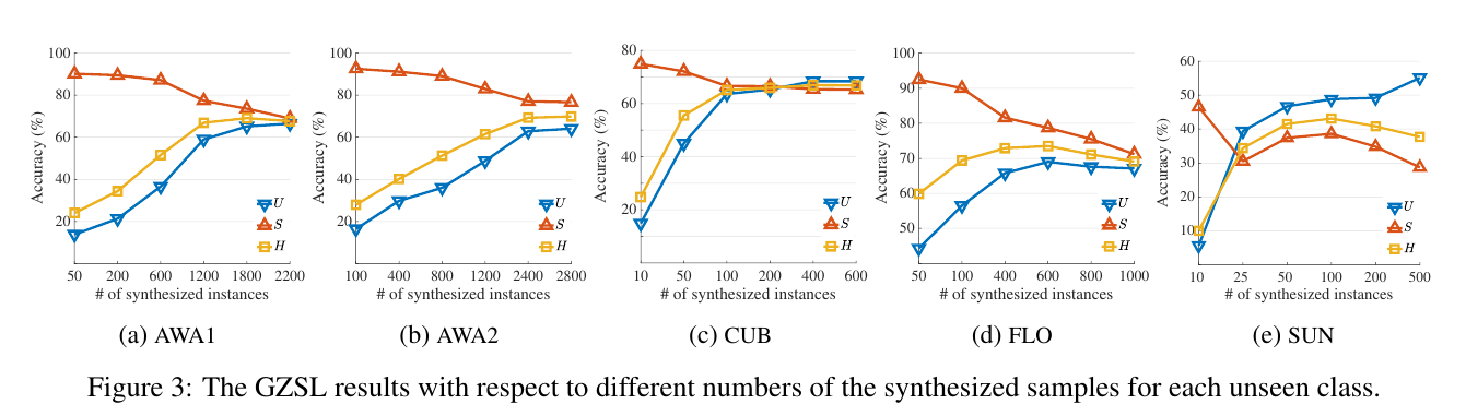
The GZSL results with respect to different numbers of the synthesized samples for each unseen class.
GZSL은 보이지 않는 각 클래스에 대해 합성된 샘플의 다른 수에 대한 결과입니다.

---

4.3 Hyper-Parameter Analysis

We evaluate the effect of different numbers of synthesized instances per unseen classes as shown in Figure 3.
우리는 그림 3과 같이 보이지 않는 클래스당 합성된 인스턴스의 다른 수의 효과를 평가합니다.

The performances on five datasets increase along with the number of synthesized examples, which shows the data-imbalance problem has been relieved by the generation model in our hybrid GZSL framework.
5개의 데이터 세트에 대한 성능은 합성된 예제의 수와 함께 증가하며, 이는 데이터 불균형 문제가 하이브리드 GZSL 프레임워크의 생성 모델에 의해 완화되었음을 보여줍니다.

Our method achieves the best results on AWA1, AWA2, CUB, FLO, and SUN when we synthesize 1,800, 2,400, 300, 600, and 100 examples per unseen classes, respectively.
우리의 방법은 보이지 않는 클래스당 각각 1,800, 2,400, 300, 600 및 100개의 예제를 합성할 때 AWA1, AWA2, CUB, FLO 및 SUN에서 최상의 결과를 얻습니다.

---

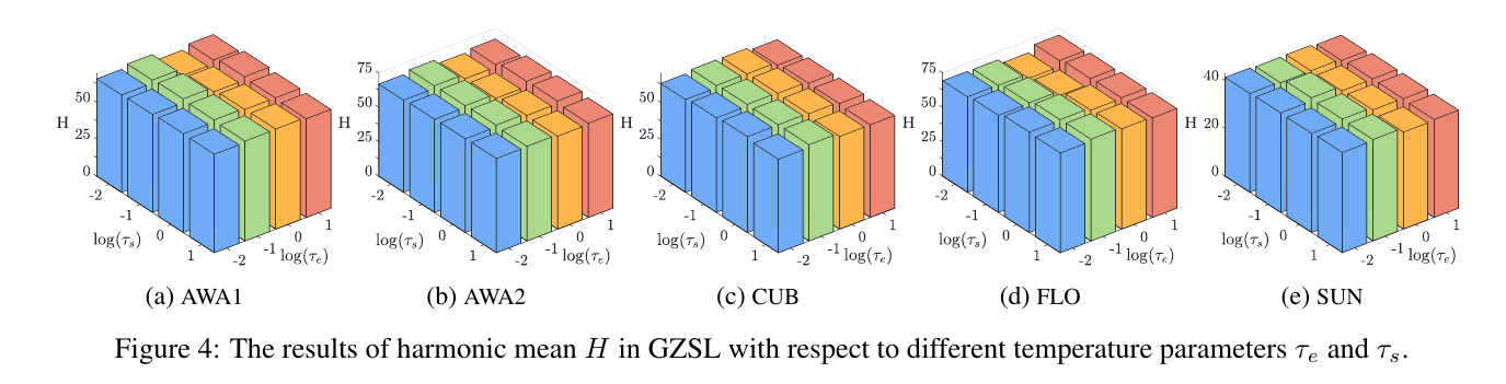
The results of harmonic mean H in GZSL with respect to different temperature parameters $τ_e$ and $τ_s$ .
다른 온도 매개변수 $τ_e$ 및 $τ_s$ 에 대한 GZSL의 조화 평균 H의 결과입니다.

---

Next, we evaluate the influence of the temperature parameters, $τ_e$ and $τ_s$ , in the contrastive embedding model.
다음으로, 대조 임베딩 모델에서 온도 매개변수 $τ_e$ 및 $τ_s$ 의 영향을 평가합니다.

We cross-validate $τ_e$ and $τ_s$ in [0.01, 0.1, 1.0, 10.0] and plot the H values with respect to different $τ_e$ and $τ_s$ , as shown in Figure 4.
[0.01, 0.1, 1.0, 10.0]에서 $τ_e$ 와 $τ_s$를 교차 검증하고 그림 4와 같이 다른 $τ_e$ 와 $τ_s$ 에 대해 H 값을 플로팅합니다.

On AWA1, CUB and SUN, our method achieves the best results when $τ_e$ = 0.1 and $τ_s$ = 0.1.
AWA1, CUB 및 SUN에서 우리의 방법은 τ e = 0.1 및 τ s = 0.1일 때 최상의 결과를 얻습니다.

On AWA2, our method achieves the best result when $τ_e$ = 10.0 and $τ_s$ = 1.0. On FLO, our method achieves the best result when $τ_e$ = 0.1 and $τ_s$ = 1.0.
AWA2에서 우리의 방법은 $τ_e$ = 10.0 및 $τ_s$ = 1.0일 때 최상의 결과를 얻습니다. FLO에서 우리의 방법은 $τ_e$ = 0.1 및 $τ_s$ = 1.0일 때 최상의 결과를 얻습니다.

---

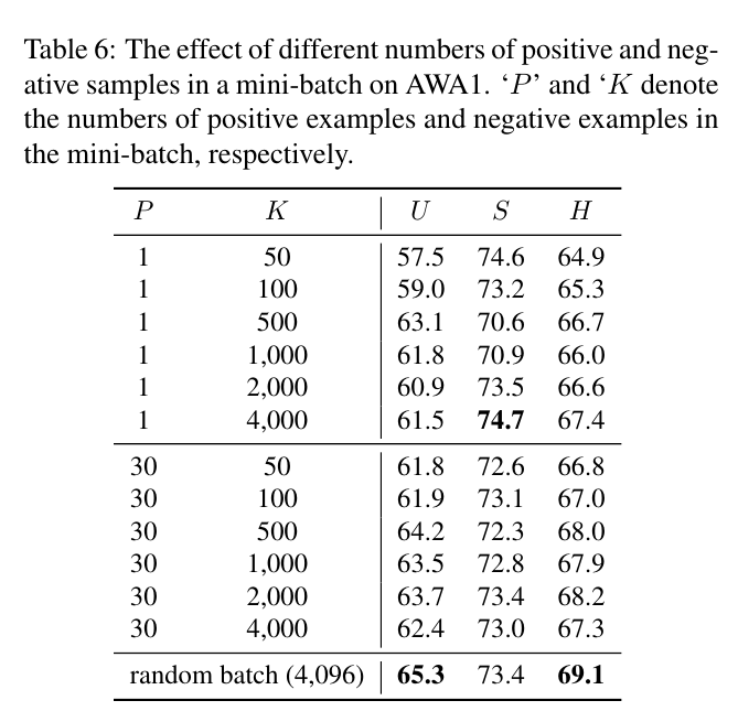
The effect of different numbers of positive and negative samples in a mini-batch on AWA1. ‘P ’ and ‘K' denote the numbers of positive examples and negative examples in the mini-batch, respectively
AWA1에 대한 미니 배치의 다양한 수의 양성 및 음성 샘플의 효과. 'P'와 'K'는 각각 mini-batch에서 긍정적인 예와 부정적인 예의 수를 나타냅니다.

---

We further evaluate the effect of the numbers of positive and negative examples in the mini-batch.
우리는 미니 배치에서 긍정적이고 부정적인 예의 수의 효과를 추가로 평가합니다.

In a mini-batch, we sample P positive examples and K negative examples for a given example.
미니 배치에서 우리는 주어진 예에 대해 P개의 긍정적인 예와 K개의 부정적인 예를 샘플링합니다.

We report the results on AWA1 in Table 6. We can observe that our method benefits from more positive examples and more negative examples.
우리는 AWA1에 대한 결과를 표 6에 보고합니다. 우리의 방법이 더 긍정적인 예와 더 많은 부정적인 예에서 이점이 있음을 관찰할 수 있습니다.

We find that using a large random batch (4,096) without a hand-crafted designed sampling strategy leads to the best results.
수작업으로 설계된 샘플링 전략 없이 대규모 무작위 배치(4,096)를 사용하는 것이 최상의 결과를 가져온다는 것을 발견했습니다.

The reason is that a large batch will contain enough positive examples and negative examples.
그 이유는 큰 배치에는 긍정적인 예와 부정적인 예가 충분히 포함될 것이기 때문입니다.

The experimental results regarding the different dimensions of the embedding space can be found in the supplementary material.
regarding ~관하여
삽입 공간의 다른 치수에 대한 실험 결과는 보충 자료에서 찾을 수 있습니다.

---