5.4 Transfer learning: Performance on downstream tasks
Although DeiT perform very well on ImageNet it is important to evaluate them on other datasets with transfer learning in order to measure the power of generalization of DeiT.
DeiT가 ImageNet에서 매우 잘 수행되지만 DeiT의 일반화 능력을 측정하기 위해 전이 학습을 사용하여 다른 데이터 세트에서 이를 평가하는 것이 중요합니다.
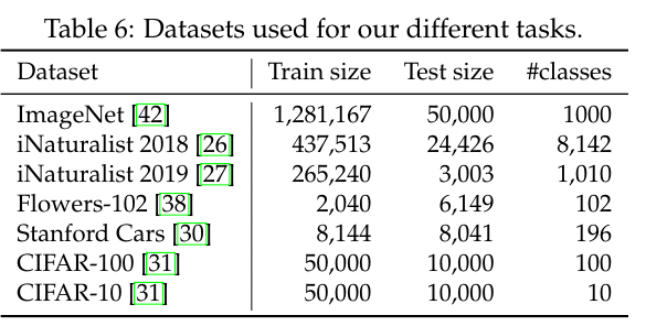
We evaluated this on transfer learning tasks by fine-tuning on the datasets in Table 6.
표 6의 데이터 세트를 미세 조정하여 전이 학습 작업에서 이를 평가했습니다.
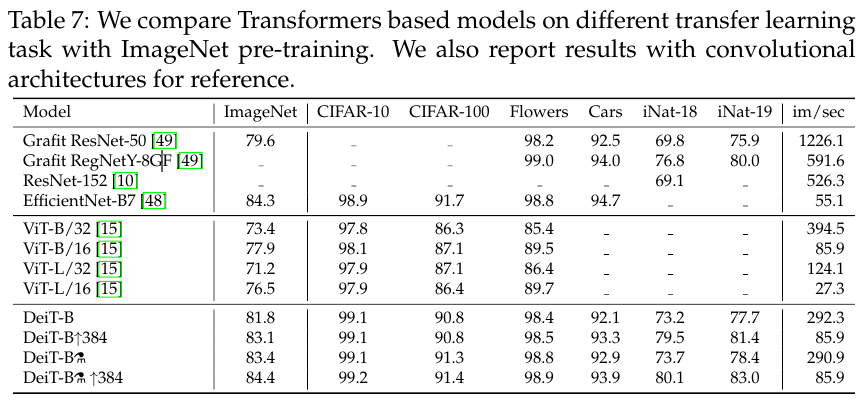
Table 7 compares DeiT transfer learning results to those of ViT [15] and state of the art convolutional architectures [48].
표 7은 DeiT 전이 학습 결과를 ViT[15] 및 최첨단 컨볼루션 아키텍처[48]의 결과와 비교합니다.
DeiT is on par with competitive convet models, which is in line with our previous conclusion on ImageNet.
in on par 동등하다 is in line with ~와 일치하다
DeiT는 ImageNet에 대한 이전의 결론과 일치하는 경쟁 컨넷 모델과 동등합니다.
Comparison vs training from scratch.
scartch 처음부터
We investigate the performance when training from scratch on a small dataset, without Imagenet pre-training.
Imagenet 사전 교육 없이 작은 데이터 세트에서 처음부터 학습할 때 성능을 조사합니다.
We get the following results on the small CIFAR-10, which is small both w.r.t. the number of images and labels:
w.r.t. ~에 대해
우리는 작은 CIFAR-10에서 다음과 같은 결과를 얻습니다.이 CIFAR-10은 이미지와 레이블의 수를 모두 줄입니다.
For this experiment, we tried we get as close as possible to the Imagenet pre-training counterpart, meaning that (1) we consider longer training schedules (up to 7200 epochs, which corresponds to 300 Imagenet epochs) so that the network has been fed a comparable number of images in total; (2) we rescale images to 224 × 224 to ensure that we have the same augmentation.
counterpart 상대 comparable 비슷한, 비교할만한
이 실험을 위해 우리는 Imagenet 사전 훈련 상대에 가능한 한 가깝게 만들려고 시도했는데, 이는 (1) 더 긴 훈련 일정 (최대 7200 개의 에포크, 300 개의 Imagenet 에포크에 해당)을 고려하여 네트워크에 비슷한 수의 이미지가 공급되었음을 의미합니다. (2) 동일한 확대를 보장하기 위해 이미지를 224 × 224로 다시 조정합니다.
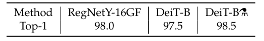
The results are not as good as with Imagenet pre-training (98.5% vs 99.1%), which is expected since the network has seen a much lower diversity.
결과는 Imagenet 사전 훈련(98.5% 대 99.1%)만큼 좋지 않습니다. 이는 네트워크가 훨씬 더 낮은 다양성을 보았기 때문에 예상되는 결과입니다.
However they show that it is possible to learn a reasonable transformer on CIFAR-10 only.
그러나 그들은 CIFAR-10에서만 합리적인 변환기를 배울 수 있음을 보여줍니다.
6. Training detils & alation
In this section we discuss the DeiT training strategy to learn vision transformers in a data-efficient manner.
이 섹션에서는 데이터 효율적인 방식으로 비전 변환기를 학습하기 위한 DeiT 교육 전략에 대해 논의합니다.
We build upon PyTorch [39] and the timm library [55] 2 .
2 The timm implementation already included a training procedure that improved the accuracy of ViT-B from 77.91% to 79.35% top-1, and trained on Imagenet-1k with a 8xV100 GPU machine.
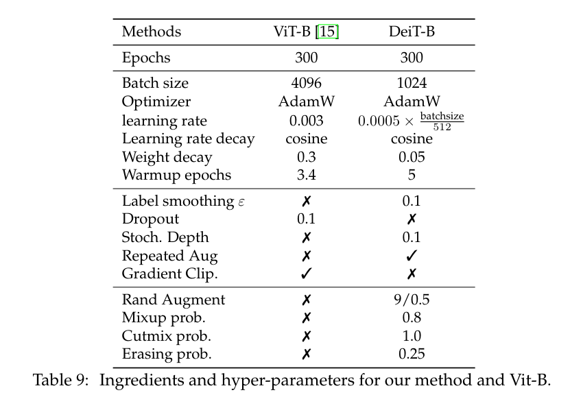
We provide hyper-parameters as well as an ablation study in which we analyze the impact of each choice.
우리는 각 선택의 영향을 분석하는 절제 연구 뿐만 아니라 하이퍼 매개변수를 제공합니다.
Initialization and hyper-parameters.
Transformers are relatively sensitive to initialization.
변압기는 초기화에 상대적으로 민감합니다.
After testing several options in preliminary experiments, some of them not converging, we follow the recommendation of Hanin and Rolnick [20] to initialize the weights with a truncated normal distribution.
preliminary 예비의 truncate 잘리다
예비 실험에서 몇 가지 옵션을 테스트한 후, 그 중 일부는 수렴되지 않습니다. Hanin and Rolnick [20]의 권장 사항에 따라 잘린 정규 분포로 가중치를 초기화합니다.
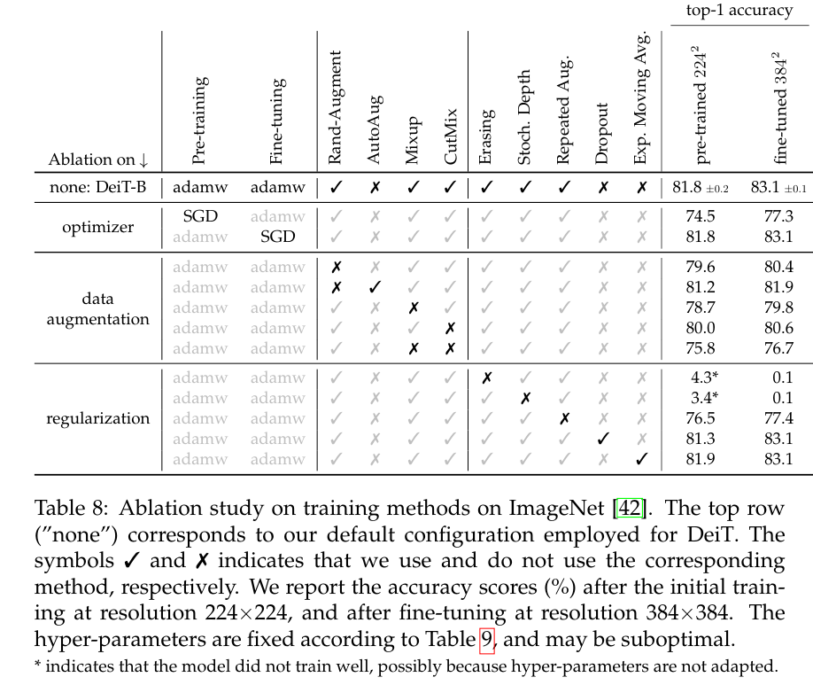
*indicates that the model did not train well, possibly because hyper-parameters are not adapted.
*는 모델이 잘 훈련되지 않았음을 나타냅니다. 아마도 하이퍼 매개변수가 적용되지 않았기 때문일 수 있습니다.
indicate 나타내다 configuration 배열, 행
Data-Augmentation.
Compared to models that integrate more priors (such as convolutions), transformers require a larger amount of data.
더 많은 이전 모델(예: 컨볼루션)을 통합하는 모델과 비교했을 때, 변압기는 더 많은 양의 데이터를 필요로 한다.
Thus, in order to train with datasets of the same size, we rely on extensive data augmentation.
따라서 동일한 크기의 데이터 세트로 훈련하기 위해 광범위한 데이터 증강에 의존합니다.
We evaluate different types of strong data augmentation, with the objective to reach a data-efficient training regime.
regime 체제 정권
데이터 효율적인 교육 체제에 도달하기 위한 목적으로 다양한 유형의 강력한 데이터 증강을 평가합니다.
Auto-Augment [11], Rand-Augment [12], and random erasing [62] improve the results.
For the two latter we use the timm [55] customizations, and after ablation we choose Rand-Augment instead of AutoAugment.
For the two latter 후자의 경우
후자의 경우 timm [55] 사용자 지정을 사용하고 절제 후에는 AutoAugment 대신 Rand-Augment을 선택합니다.
Overall our experiments confirm that transformers require a strong data augmentation:
전반적으로 우리의 실험은 변압기가 강력한 데이터 증강을 필요로한다는 것을 확인합니다.
almost all the data-augmentation methods that we evaluate prove to be useful.
우리가 평가하는 거의 모든 데이터 증강 방법이 유용하다는 것이 입증되었습니다.
One exception is dropout, which we exclude from our training procedure.
한 가지 예외는 drou out이며 training 절차에서 제외합니다.
Regularization & Optimizers.
We have considered different optimizers and cross-validated different learning rates and weight decays.
우리는 다양한 옵티마이저를 고려하고 다양한 학습률과 가중치 감쇠를 교차 검증했습니다.
Transformers are sensitive to the setting of optimization hyper-parameters.
변압기는 최적화 하이퍼 매개변수 설정에 민감합니다.
Therefore, during cross-validation, we tried 3 different learning rates ( , , ) and 3 weight decay (0.03, 0.04, 0.05).
따라서 교차 검증 동안 3개의 다른 학습률(5.10 -4 , 3.10 -4 , 5.10 -5 )과 3개의 가중치 감쇠(0.03, 0.04, 0.05)를 시도했습니다.\
We scale the learning rate according to the batch size with the formula: '' = × batchsize, similarly to Goyal et al. [19] except that we use 512 instead of 256 as the base value.
Goyal et al.과 유사하게 'lr scaled' = 'lr 512' × batchsize 공식을 사용하여 배치 크기에 따라 학습률을 조정합니다. [19] 기본 값으로 256 대신 512를 사용한다는 점을 제외하고.
The best results use the AdamW optimizer with the same learning rates as ViT [15] but with a much smaller weight decay, as the weight decay reported in the paper hurts the convergence in our setting.
최상의 결과는 ViT[15]와 동일한 학습률을 갖지만 훨씬 더 작은 가중치 감쇠를 갖는 AdamW 최적화 프로그램을 사용하는 것입니다. 논문에서 보고된 가중치 감소가 우리 설정의 수렴을 손상시키기 때문입니다.
We have employed stochastic depth [29], which facilitates the convergence of transformers, especially deep ones [16, 17].
stochastic 확률론적인 facilitates 가능하게 하다
우리는 트랜스포머, 특히 깊은 트랜스포머의 수렴을 용이하게 하는 확률론적 깊이[29]를 사용했습니다[16, 17].
For vision transformers, they were first adopted in the training procedure by Wightman [55].
비전 변압기의 경우 Wightman[55]의 훈련 절차에서 처음으로 채택했습니다.
Regularization like Mixup [60] and Cutmix [59] improve performance.
Mixup [60] 및 Cutmix [59]와 같은 정규화는 성능을 향상시킵니다.
We also use repeated augmentation [4, 25], which provides a significant boost in performance and is one of the key ingredients of our proposed training procedure.
우리는 또한 성능에 상당한 향상을 제공하고 제안된 훈련 절차의 핵심 요소 중 하나인 반복적인 증강[4, 25]을 사용합니다.
Exponential Moving Average (EMA).
지수 이동 평균(EMA)
We evaluate the EMA of our network obtained after training.
교육 후 얻은 네트워크의 EMA를 평가합니다.
There are small gains, which vanish after fine-tuning:
미세 조정 후에 사라지는 작은 이득이 있습니다.
the EMA model has an edge of is 0.1 accuracy points, but when fine-tuned the two models reach the same (improved) performance.
EMA 모델의 가장자리는 0.1 정확도 포인트이지만 미세 조정하면 두 모델이 동일한(향상된) 성능에 도달합니다.
Fine-tuning at different resolution.
다른 해상도에서 미세 조정.
We adopt the fine-tuning procedure from Touvron et al. [51]:
우리는 Touvron 등의 미세 조정 절차를 채택합니다.
our schedule, regularization and optimization procedure are identical to that of FixEfficientNet but we keep the training-time data augmentation (contrary to the dampened data augmentation of Touvron et al. [51]).
우리의 일정, 정규화 및 최적화 절차는 FixEfficientNet의 것과 동일하지만 훈련 시간 데이터 증대를 유지합니다(Touvron et al.[51]의 감쇠 데이터 증대와 반대).
We also interpolate the positional embeddings:
interpolate 보간하다
우리는 또한 위치 임베딩을 보간합니다:
In principle any classical image scaling technique, like bilinear interpolation, could be used.
원칙적으로 쌍선형 보간(bilinear interpolation)과 같은 모든 기존 이미지 스케일링 기술을 사용할 수 있습니다.
However, a bilinear interpolation of a vector from its neighbors reduces its -norm compared to its neighbors.
그러나 이웃 벡터의 쌍선형 보간은 이웃에 비해 'l2 -norm'을 줄입니다.
These low-norm vectors are not adapted to the pre-trained transformers and we observe a significant drop in accuracy if we employ use directly without any form of fine-tuning.
이러한 low-norm 벡터는 사전 훈련된 변압기에 적용되지 않으며 어떤 형태의 미세 조정 없이 직접 사용하면 정확도가 크게 떨어지는 것을 관찰할 수 있습니다.
Therefore we adopt a bicubic interpolation that approximately preserves the norm of the vectors, before fine-tuning the network with either AdamW [36] or SGD.
bicubic 쌍입방(바이큐빅)
따라서 AdamW [36] 또는 SGD로 네트워크를 미세 조정하기 전에 벡터의 노름을 대략적으로 유지하는 쌍삼차 보간법을 채택합니다.
These optimizers have a similar performance for the fine-tuning stage, see Table 8.
By default and similar to ViT [15] we train DeiT models with at resolution 224 and we fine-tune at resolution 384.
기본적으로 ViT[15]와 유사하게 해상도 224에서 DeiT 모델을 훈련하고 해상도 384에서 미세 조정합니다.
We detail how to do this interpolation in Section 3.
detail 자세히 설명하다
However, in order to measure the influence of the resolution we have finetuned DeiT at different resolutions.
그러나 해상도의 영향을 측정하기 위해 DeiT를 다양한 해상도에서 미세 조정했습니다.
We report these results in Table 10.
Training time.
A typical training of 300 epochs takes 37 hours with 2 nodes or 53 hours on a single node for the DeiT-B.
As a comparison point, a similar training with a RegNetY-16GF [40] (84M parameters) is 20% slower.
DeiT-S and DeiT-Ti are trained in less than 3 days on 4 GPU.
Then, optionally we fine-tune the model at a larger resolution.
그런 다음 선택적으로 모델을 더 큰 해상도로 미세 조정합니다.
This takes 20 hours on a single node (8 GPU) to produce a FixDeiT-B model at resolution 384×384, which corresponds to 25 epochs.
corresponds 일치하다, 부합하다
Not having to rely on batch-norm allows one to reduce the batch size without impacting performance, which makes it easier to train larger models.
impact 영향을 주다
batch-norm에 의존할 필요가 없기 때문에 성능에 영향을 주지 않고 배치 크기를 줄일 수 있으므로 더 큰 모델을 더 쉽게 훈련할 수 있습니다.
Note that, since we use repeated augmentation [4, 25] with 3 repetitions, we only see one third of the images during a single epoch 3 .
3번의 반복으로 반복된 증대[4, 25]를 사용하기 때문에 단일 epoch 3 동안 이미지의 1/3만 봅니다.