[Optimizer]Stochastic Gradient Descent

우선 GD의 한계점부터 보자.

GD의 경우 local minimum에서 빠져나올 수 없기때문에 시작위치가 매우 중요하다.

import numpy as np
import matplotlib.pyplot as plt

# Gradient Descent 알고리즘 구현
def gradient_descent(function, derivative, start_point, lr, iterations=100):
    x = start_point
    history = [x]
    for _ in range(iterations):
        x = x - lr * derivative(x)
        history.append(x)
    return np.array(history)

# 주어진 함수와 도함수 정의
def f(x):
    return x * (x - 1) * (x - 2) * (x - 4)

def df(x):
    return 4 * x**3 - 21 * x**2 + 22 * x - 4

# 시작점, 학습률, 반복 횟수 설정
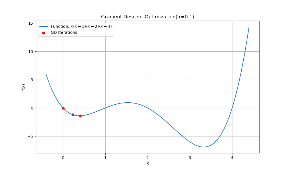
start_point = 0
lr = 0.1
iterations = 3

# Gradient Descent 수행
x_history = gradient_descent(f, df, start_point, lr, iterations)

# 함수와 GD 과정 시각화
x_values = np.linspace(-0.4, 4.4, 400)
y_values = f(x_values)

plt.figure(figsize=(10, 6))
plt.plot(x_values, y_values, label="Function: $x(x-1)(x-2)(x-4)$")
plt.scatter(x_history, f(x_history), color='red', label="GD Iterations")
plt.title(f"Gradient Descent Optimization(lr={lr})")
plt.xlabel("x")
plt.ylabel("f(x)")
plt.legend()
plt.grid(True)
plt.show()

• lr을 0.1로 하는 경우
  

• lr을 0.2로 하는 경우
  

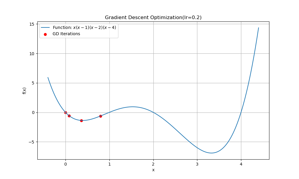
진동하다가 수렴

• lr을 0.4로 하는 경우
  

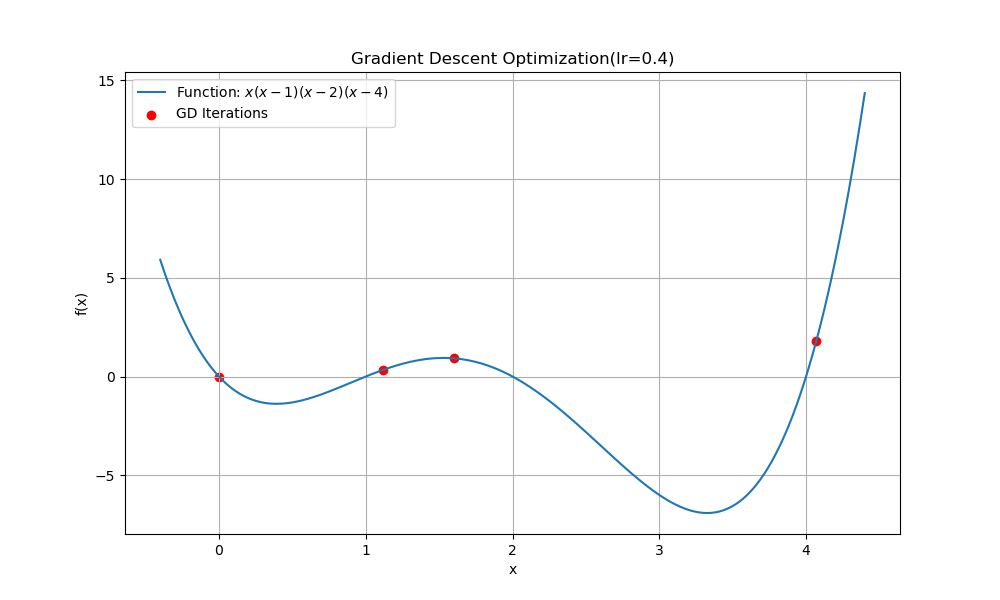
수렴이 아니라 overshoot 하는 모습을 볼 수 있다.

느리다.

• object function을 계산할때, 모든 loss를 고려하기 때문에 object function 계산에 많은 시간이 소요된다.

SGD의 경우 이러한 단점을 개선할 수 있다.

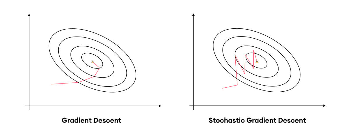
• loss계산에 있어 무작위 샘플을 진행하여 오류의 기울기를 계산한다.
  • 무작위 샘플에 대한 loss계산을 반복하여 결론적으로는 minimum값에 최적화된다.
  • 더 많은 epoch를 반복하더라도 하나의 계산에 대한 시간이 훨씬 짧기 때문에 결론적으로 GD보다 적은 시간이 걸린다.
• 무작위 샘플로 loss를 계산하기 때문에 local minimum을 벗어날 기회가 있다.
  • global minimum을 찾아간다는 뜻은 아니다.

SGD는 GD의 object function 계산 과정에서 데이터를 stochastic하게(확률론적으로) 고려하여 계산 효율성을 높혔다.