[데이터분석]Bootstrap, 심슨의 역설

민서·2024년 4월 19일

데이터분석 파이썬

데이터분석

목록 보기

6/11

이항 분포(Binomial Distribution)

저번 게시물에 정리했던 이항분포를 통해 문제를 계산해보자
eg. 어떤 선거에서 표본집단 100명의 투표자들에게 53%의 지지를 얻었다면, 당선될것인가?
분산 = 0.53*0.47=0.2491
표준편차 = sqrt(0.2491) = 0.4991
standard_error = 0.4991/sqrt(100)=0.0499(약 5%)
당선확률을 53%+-5%정도로 볼 수 있다.
위에 예시는 표본집단의 확률과 시행횟수를 통해 모집단의 평균을 추정했다.

만약 95%의 신뢰구간을 얻고싶다면, 당선확률을 53%+-10%정도로 볼 수 있다.

부트스트랩(Bootstrap)

부트스트랩 정의

재표집(resampling)을 통해 통계적 추정치의 분포를 추정하는 방법이다.
재표집(Resampling): 기존의 표본 데이터 세트에서 복원 추출 방식을 사용하여, 원래 표본과 같은 크기의 새로운 표본을 여러 번 생성합니다. 복원 추출이란 한 번 선택된 데이터를 다시 선택할 수 있도록 다시 표본집단에 반환하는 방식이다.
통계량 계산: 각각의 재표집된 표본에 대해 원하는 통계량(평균, 분산 등)을 계산한다.
분포 추정: 계산된 통계량들의 분포를 사용하여 모집단의 해당 통계량에 대한 추정치를 도출한다. 이 분포로부터 신뢰 구간이나 기타 통계적 결론을 도출할 수 있다.

부트스트랩의 사용

부트스트랩은 모집단의 실제 분포에 대한 가정이 필요 없기 때문에, 다양한 통계적 상황에서 유용하게 사용된다. 특히 표본 크기가 작거나, 복잡한 통계 모델에서 모수의 신뢰 구간을 추정할 때 효과적이다.

왜 부트스트랩이 유효한가?

부트스트랩은 원래의 표본이 모집단을 잘 대표한다는 가정 하에 작동한다. 복원 추출 방식으로 '새로운' 표본을 만들어내며, 이론적으로는 이 표본들이 모집단에서 추출될 수 있었을 것이라고 가정한다. 이를 통해, 실제 모집단을 사용하지 않고도 통계량의 샘플링 분포를 추정할 수 있다. 이는 모집단에 대한 강한 가정 없이도 통계적 추론을 가능하게 한다.

부트스트랩의 장점

유연성(Flexibility)
다양한 통계량과 복잡한 추정기에 적용할 수 있다.
단순성(Simplicity)
복잡한 수학적 공식을 필요로 하지 않으면서도 쉽게 구현하고 이해할 수 있다.
적용성(Applicability)
전통적인 매개변수적 방법을 사용하기 어려운 경우(예: 표본 크기가 너무 작거나 모집단의 분포가 알려지지 않은 경우)에 유용하다.

부트스트랩의 한계
정확성(Accuracy)
원래 표본이 모집단을 대표하지 않는 경우 부트스트랩 추정의 정확성이 떨어질 수 있다. 즉, 표본이 편향되어 있거나 모집단의 특성을 제대로 반영하지 못하면 부트스트랩 결과도 오류를 포함할 가능성이 커진다.
계산 강도(Computationally Intensive)
부트스트랩은 많은 계산을 요구하며, 표본 크기나 부트스트랩 샘플의 수가 증가할수록 계산 부담이 커진다. 따라서 컴퓨터 자원을 많이 소모할 수 있다.

응용 예시
부트스트랩을 사용하여 평균 키 차이를 분석하거나, 특정 그룹(커피를 마시는 사람들과 마시지 않는 사람들) 사이의 평균 키 차이를 분석한다.

데이터 분석 실습

import pandas as pd
import numpy as np
np.random.seed(104)
df = pd.read_csv('data/MDA_09_coffee_dataset.csv')
print(df.info())
print(df.head(5))

# Randomly sample 200 samples from the population.
df_sample = df.sample(200)
print(df_sample.info())
print(df_sample.head())

##### Confidence interval using bootstrap #####
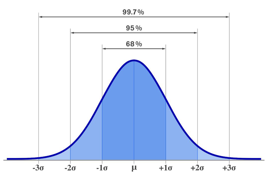
# Let's repeat the bootstrap 10,000 times to find the 99.7% confidence interval for the height difference
# between people who do not drink coffee and people who drink coffee.
# 1. Average height difference between non-coffee drinkers and coffee drinkers
iterationNum = 10000
diffHeightList = []
for _ in range(iterationNum):
    bootSample = df_sample.sample(200, replace=True) # 복원 추출(뺀게 사라지지 않음)
    nonCoffeeHeightMean = bootSample[bootSample['drinks_coffee'] == False].height.mean()
    # Avg. height of people who drink coffee
    coffeeHeightMean = bootSample[bootSample['drinks_coffee'] == True].height.mean()
    diff = nonCoffeeHeightMean - coffeeHeightMean
    diffHeightList.append(diff)
print(diffHeightList)

print("mean of height diff:", np.mean(diffHeightList))
print("SE of Height diff:", np.std(diffHeightList))
print("Lowerbound(0.3):", np.percentile(diffHeightList, 0.3))
print("Uppperbound(99.7):", np.percentile(diffHeightList, 99.7))

실제 모집단이 잘 모사되었는지 확인

print("##### Height differences in the population #####")
# # 1. Average height difference between non-coffee drinkers and coffee drinkers
diffHeight = df[df['drinks_coffee'] == False].height.mean() - df[df['drinks_coffee'] == True].height.mean()
print("diffHeight : ",diffHeight)

print("Lowerbound(0.3):", np.percentile(diffHeightList, 0.3))
print("Uppperbound(99.7):", np.percentile(diffHeightList, 99.7))

커피를 많이 마신 집단이 키가 더 큰게 과연 타당한가?

심슨의 역설(Simpson's Paradox)

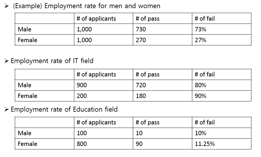
심슨의 역설 정의: 복수의 그룹에 걸쳐 데이터를 분석할 때 보이는 경향성이 전체 데이터를 합쳤을 때와 달라지는 현상이다.

예시: 특정 직업군(예: IT와 교육 분야)에서 성별에 따른 취업률을 분석할 때, 각각의 직업군에서 보이는 성별 취업률 차이가 전체를 합쳤을 때와는 다르게 나타날 수 있다.

코드 확인

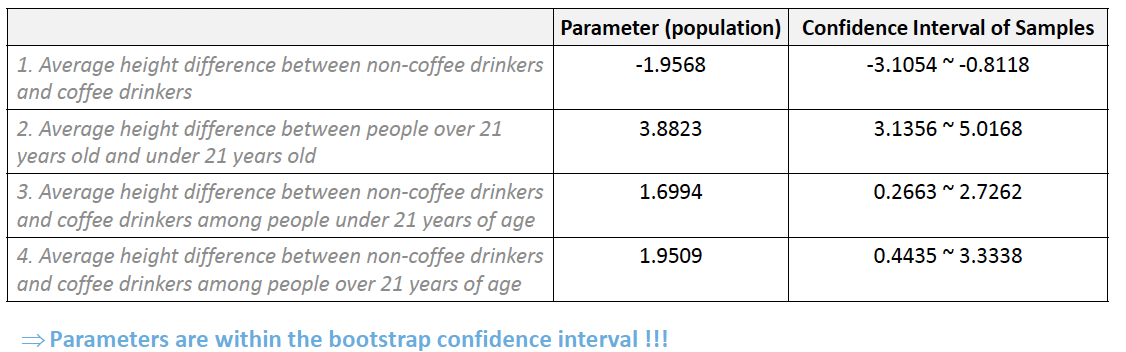
# 2. Average height difference between people over 21 years old and under 21 years old
diffHeightListByAge = []
for _ in range(iterationNum):
    bootSample = df_sample.sample(200, replace=True) # sampling with replacement
    over21HeightMean = bootSample[bootSample['age'] == '>=21'].height.mean() # Avg.Height for over 21
    under21HeightMean = bootSample[bootSample['age'] == '<21'].height.mean() # Avg.Height for under 21
    diff = over21HeightMean - under21HeightMean
    diffHeightListByAge.append(diff)
# When the confidence level is 99%.7, the confidence interval for the average height difference
print("Lowerbound(0.3):", np.percentile(diffHeightListByAge, 0.3))
print("Uppperbound(99.7):", np.percentile(diffHeightListByAge, 99.7))

# 3. Average height difference between non-coffee drinkers and coffee drinkers among people under 21 years of age
diffHeightListUnder21 = []
for _ in range(iterationNum):
    bootSample = df_sample.sample(200, replace=True) # sampling with replacement
    # Average height of people under 21 years of age who do not drink coffee
    nonCoffeeHeightMeanUnder21 = bootSample.query("age == '<21' and drinks_coffee == False").height.mean()
    # Average height of people under 21 years of age who drink coffee
    coffeeHeightMeanUnder21 = bootSample.query("age == '<21' and drinks_coffee == True").height.mean()
    diff = nonCoffeeHeightMeanUnder21 - coffeeHeightMeanUnder21
    diffHeightListUnder21.append(diff)
# When the confidence level is 99%.7, the confidence interval for the average height difference
print("Lowerbound(0.3):", np.percentile(diffHeightListUnder21, 0.3))
print("Uppperbound(99.7):", np.percentile(diffHeightListUnder21, 99.7))

# 4. # Average height difference between non-coffee drinkers and coffee drinkers among people over 21 years of age
diffHeightListOver21 = []
for _ in range(iterationNum):
    bootSample = df_sample.sample(200, replace=True) # sampling with replacement
    # Average height of people over 21 years of age who do not drink coffee
    nonCoffeeHeightMeanOver21 = bootSample.query("age != '<21' and drinks_coffee == False").height.mean()
    # Average height of people over 21 years of age who drink coffee
    coffeeHeightMeanOver21 = bootSample.query("age != '<21' and drinks_coffee == True").height.mean()
    diff = nonCoffeeHeightMeanOver21 - coffeeHeightMeanOver21
    diffHeightListOver21.append(diff)
# When the confidence level is 99%.7, the confidence interval for the average height difference
print("Lowerbound(0.3):", np.percentile(diffHeightListOver21, 0.3))
print("Uppperbound(99.7):", np.percentile(diffHeightListOver21, 99.7))

->커피를 마신 그룹의 키가 더 컸지만, 21세 이상과 이하로 나누어봤을떄 두 집단 모두 커피를 안마신 그룹의 키가 더 큼을 확인할 수 있다.(심슨의 역설)

print("##### Height differences in the population #####")
# # 1. Average height difference between non-coffee drinkers and coffee drinkers
diffHeight = df[df['drinks_coffee'] == False].height.mean() - df[df['drinks_coffee'] == True].height.mean()
print("1. diffHeight : ",diffHeight)
# 2. Average height difference between people over 21 years old and under 21 years old
diffHeightByAge = df[df['age'] == '>=21'].height.mean() - df[df['age'] == '<21'].height.mean()
print("2. diffHeight : ",diffHeightByAge)
# 3. Average height difference between non-coffee drinkers and coffee drinkers among people under 21 years of age
diffHeightUnder21 = df.query("age == '<21' and drinks_coffee == False").height.mean() - df.query("age == '<21' and drinks_coffee == True").height.mean()
print("3. diffHeight : ",diffHeightUnder21)
# 4. Average height difference between non-coffee drinkers and coffee drinkers among people over 21 years of age
diffHeightOver21 = df.query("age != '<21' and drinks_coffee == False").height.mean() - df.query("age != '<21' and drinks_coffee == True").height.mean()
print("4. diffHeight : ",diffHeightOver21)