해당 포스트는 https://www.youtube.com/@multipleobjecttracking1226중 "Part 3: Tracking a known number of objects in clutter"의 내용을 기반으로 작성되었으며, 해당 영상은 본 글에서 생략된 다양한 visualization 자료가 포함되어 있음.
1. 개요
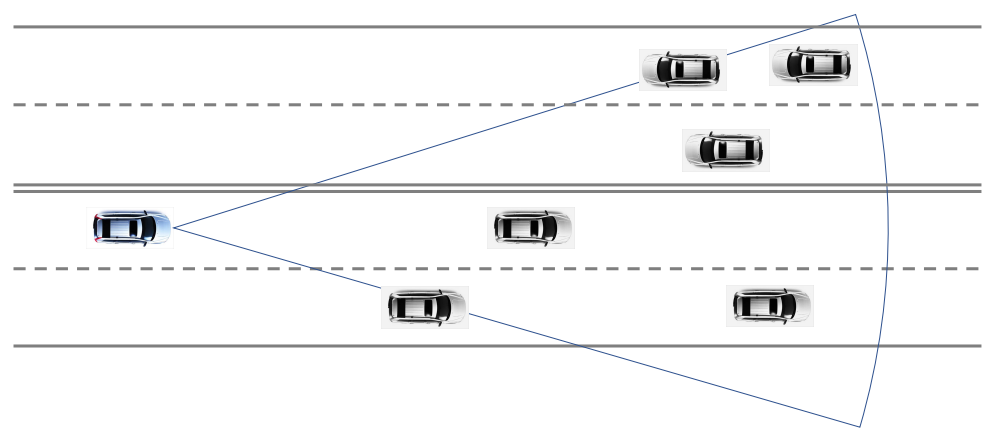
이전 글에서는 관심 객체가 하나만 등장하는 SOT를 수행했지만, 이번 글에서는 관심 객체가 n개 등장하는 상황에서 다수의 객체를 동시에 추적하는 방법을 살펴본다. 일반적인 MOT와는 달리 n의 값을 알고있다고 가정한다. 관심 객체가 여러 개 존재하기 때문에 SOT보다 data association 등이 좀 더 복잡해진다.
n개의 객체가 있다고 가정하기 때문에 state에 대한 prior는 p ( X 0 ) = p ( x 0 1 , ⋯ , x 0 n ) p(X_0) = p(x_0^1, \cdots, x_0^n ) p ( X 0 ) = p ( x 0 1 , ⋯ , x 0 n )
p ( X ) = p ( x 1 , ⋯ , x n ) = ∏ i = 1 n p i ( x i ) \begin{aligned} p(X) & = p(x^1, \cdots, x^n ) \\ & = \prod^n_{i=1}{p^i(x^i)} \end{aligned} p ( X ) = p ( x 1 , ⋯ , x n ) = i = 1 ∏ n p i ( x i ) 그리고 만약 확률 분포가 여러 분포의 합으로 이루어진 mixture density라면 다음과 같이 쓸 수 있다.
p ( X ) = ∑ h w h ∏ i = 1 n p i , h ( x i ) \begin{aligned} p(X) & = \sum_h w^h \prod^n_{i=1}{p^{i, h}(x^i)} \end{aligned} p ( X ) = h ∑ w h i = 1 ∏ n p i , h ( x i ) 2. Modeling the Mearsurements
우선 여러 객체가 있을 때의 data association 표현을 알아보자. SOT 때과 비슷하지만, 몇 가지 추가되는 조건이 생긴다. 먼저 기본적으로 data association Θ k \Theta_k Θ k k k k θ k \theta_k θ k θ k \theta_k θ k
θ k i = { j i f o b j e c t i a s s o c i a t e d t o m e a s u r e m e n t j 0 i f o b j e c t i i s u n d e t e c t e d \theta^i_k = \begin{cases} j \;\;\;\;\;\; if \; object \; i \; associated \; to \; measurement \; j\\ 0 \;\;\;\;\;\; if \; object \; i \; is \; undetected \end{cases} θ k i = { j i f o b j e c t i a s s o c i a t e d t o m e a s u r e m e n t j 0 i f o b j e c t i i s u n d e t e c t e d θ k = [ θ k 1 , ⋯ , θ k n ] \theta_k = [ \theta^1_k , \cdots , \theta ^n_k ] θ k = [ θ k 1 , ⋯ , θ k n ] 예를 들어 객체가 2개 X = [ x 1 , x 2 ] X=[x^1, x^2] X = [ x 1 , x 2 ] Z = [ z 1 , z 2 ] Z=[z^1, z^2] Z = [ z 1 , z 2 ] θ = [ θ 1 . θ 2 ] = [ 2 , 0 ] \theta =[\theta^1. \theta^2] = [2,0] θ = [ θ 1 . θ 2 ] = [ 2 , 0 ] z 2 z^2 z 2
객체를 측정값 z z z θ k i ∈ { 0 , ⋯ , m k } \theta^i_k \in \{0, \cdots, m_k \} θ k i ∈ { 0 , ⋯ , m k } m k m_k m k m k c = m k − m k o m_k^c = m_k - m_k^o m k c = m k − m k o
이를 이용하여 우리는 필터의 업데이트 단계를 위한 measurement likelihood, p Z ∣ X ( Z ∣ X ) p_{Z|X}(Z|X) p Z ∣ X ( Z ∣ X )
p Z ∣ X ( Z ∣ X ) = ∑ θ ∈ Θ p Z , θ ∣ X ( Z , θ ∣ X ) = ∑ θ ∈ Θ p Z ∣ X , θ , m ( Z ∣ X , θ , m ) p θ , m ∣ X ( θ , m ∣ X ) p_{Z|X}(Z|X) = \sum_{\theta \in \Theta}p_{Z, \theta|X}(Z,\theta|X) = \sum_{\theta \in \Theta}p_{Z|X, \theta, m}(Z|X, \theta, m)p_{\theta, m|X}(\theta, m|X) p Z ∣ X ( Z ∣ X ) = θ ∈ Θ ∑ p Z , θ ∣ X ( Z , θ ∣ X ) = θ ∈ Θ ∑ p Z ∣ X , θ , m ( Z ∣ X , θ , m ) p θ , m ∣ X ( θ , m ∣ X ) 여기서 나타나는 각 term을 풀어쓰면 다음과 같다.
p θ , m ∣ X ( θ , m ∣ X ) = ∏ i : θ k i = 0 ( 1 − P D ( x k i ) ) ∏ i : θ k i ≠ 0 P D ( x k i ) ⏟ ( 1 ) P o ( m c ∣ λ c ˉ ) ⏟ ( 2 ) 1 ( m m o ) m o ! ⏟ ( 3 ) = m c ! m ! P o ( m c ∣ λ c ˉ ) ∏ i : θ k i = 0 ( 1 − P D ( x k i ) ) ∏ i : θ k i ≠ 0 P D ( x k i ) \begin{aligned} p_{\theta, m|X}(\theta, m|X) & = \underbrace{\prod_{i:\theta^i_k=0}{(1-P^D(x_k^i))}\prod_{i:\theta^i_k\ne0}{P^D(x_k^i)}}_{(1)} \underbrace{Po(m^c|\bar{\lambda_c})}_{(2)} \underbrace{\frac{1}{ \begin{pmatrix} m\\ m^o \end{pmatrix}m^o! }}_{(3)} \\ & = \frac{m^c!}{m!}Po(m^c|\bar{\lambda_c})\prod_{i:\theta^i_k=0}{(1-P^D(x_k^i))}\prod_{i:\theta^i_k\ne0}{P^D(x_k^i)} \end{aligned} p θ , m ∣ X ( θ , m ∣ X ) = ( 1 ) i : θ k i = 0 ∏ ( 1 − P D ( x k i ) ) i : θ k i = 0 ∏ P D ( x k i ) ( 2 ) P o ( m c ∣ λ c ˉ ) ( 3 ) ( m m o ) m o ! 1 = m ! m c ! P o ( m c ∣ λ c ˉ ) i : θ k i = 0 ∏ ( 1 − P D ( x k i ) ) i : θ k i = 0 ∏ P D ( x k i ) (1)은 m o m^o m o m c = m − m o m^c = m - m^o m c = m − m o m m m m o m^o m o
그리고 각 측정치가 독립적이라고 가정하면, 나머지 term은 다음과 같이 쓸 수 있다. 첫번째 term은 PPP에서의 spatial pdf, g는 measurement model이다.
p Z ∣ X , θ , m ( Z ∣ X , θ , m ) = ∏ j : ∄ θ i = j f c ( z j ) ∏ i : θ i ≠ 0 g ( z θ i ∣ x i ) p_{Z|X, \theta, m}(Z|X, \theta, m) = \prod_{j: \nexists \theta^i=j}{f_c(z^j)}\prod_{i: \theta^i\ne0}{g(z^{\theta^i}|x^i)} p Z ∣ X , θ , m ( Z ∣ X , θ , m ) = j : ∄ θ i = j ∏ f c ( z j ) i : θ i = 0 ∏ g ( z θ i ∣ x i ) 이 두 식을 결합하여 정리하면 다음과 같다.
p Z ∣ X ( Z ∣ X ) = ∑ θ ∈ Θ p Z , θ ∣ X ( Z , θ ∣ X ) = ∑ θ ∈ Θ p Z ∣ X , θ , m ( Z ∣ X , θ , m ) p θ , m ∣ X ( θ , m ∣ X ) = ∑ θ ∈ Θ [ ∏ j : ∄ θ i = j f c ( z j ) ∏ i : θ i ≠ 0 g ( z θ i ∣ x i ) m c ! m ! P o ( m c ∣ λ c ˉ ) ∏ i : θ i = 0 ( 1 − P D ( x i ) ) ∏ i : θ i ≠ 0 P D ( x i ) ] = ∑ θ ∈ Θ [ e − λ c ˉ m ! ∏ j : ∄ θ i = j λ c ( z j ) ∏ i : θ i = 0 ( 1 − P D ( x i ) ) ∏ i : θ i ≠ 0 P D ( x i ) g ( z θ i ∣ x i ) ] = ∑ θ ∈ Θ [ e − λ c ˉ m ! ∏ j = 1 m λ c ( z j ) ∏ i : θ i = 0 ( 1 − P D ( x i ) ) ∏ i : θ i ≠ 0 P D ( x i ) g ( z θ i ∣ x i ) λ c ( z θ i ) ] ∝ ∑ θ ∈ Θ [ ∏ i : θ i = 0 ( 1 − P D ( x i ) ) ⏟ m i s s e d d e t e c t i o n s ∏ i : θ i ≠ 0 P D ( x i ) g ( z θ i ∣ x i ) λ c ( z θ i ) ⏟ d e t e c t i o n s ] \begin{aligned} p_{Z|X}(Z|X) & = \sum_{\theta \in \Theta}p_{Z, \theta|X}(Z,\theta|X) = \sum_{\theta \in \Theta}p_{Z|X, \theta, m}(Z|X, \theta, m)p_{\theta, m|X}(\theta, m|X) \\ & = \sum_{\theta \in \Theta}\left[ \prod_{j: \nexists \theta^i=j}{f_c(z^j)}\prod_{i: \theta^i\ne0}{g(z^{\theta^i}|x^i)} \frac{m^c!}{m!}Po(m^c|\bar{\lambda_c})\prod_{i:\theta^i=0}{(1-P^D(x^i))}\prod_{i:\theta^i\ne0}{P^D(x^i)} \right] \\ & = \sum_{\theta \in \Theta} \left[ \frac{e^{-\bar{\lambda_c}}}{m!} \prod_{j: \nexists \theta^i=j} \lambda_c(z^j) \prod_{i:\theta^i=0}{(1-P^D(x^i))} \prod_{i: \theta^i\ne0}{P^D(x^i)g(z^{\theta^i}|x^i)} \right] \\ & = \sum_{\theta \in \Theta} \left[ \frac{e^{-\bar{\lambda_c}}}{m!} \prod_{j=1}^m \lambda_c(z^j) \prod_{i:\theta^i=0}{(1-P^D(x^i))} \prod_{i: \theta^i\ne0}{\frac{P^D(x^i)g(z^{\theta^i}|x^i)}{\lambda_c(z^{\theta^i})}} \right] \\ & \propto \sum_{\theta \in \Theta} \left[ \underbrace{\prod_{i:\theta^i=0}{(1-P^D(x^i))}}_{missed\;detections} \underbrace{\prod_{i: \theta^i\ne0}{\frac{P^D(x^i)g(z^{\theta^i}|x^i)}{\lambda_c(z^{\theta^i})}}}_{detections} \right] \end{aligned} p Z ∣ X ( Z ∣ X ) = θ ∈ Θ ∑ p Z , θ ∣ X ( Z , θ ∣ X ) = θ ∈ Θ ∑ p Z ∣ X , θ , m ( Z ∣ X , θ , m ) p θ , m ∣ X ( θ , m ∣ X ) = θ ∈ Θ ∑ ⎣ ⎢ ⎡ j : ∄ θ i = j ∏ f c ( z j ) i : θ i = 0 ∏ g ( z θ i ∣ x i ) m ! m c ! P o ( m c ∣ λ c ˉ ) i : θ i = 0 ∏ ( 1 − P D ( x i ) ) i : θ i = 0 ∏ P D ( x i ) ⎦ ⎥ ⎤ = θ ∈ Θ ∑ ⎣ ⎢ ⎡ m ! e − λ c ˉ j : ∄ θ i = j ∏ λ c ( z j ) i : θ i = 0 ∏ ( 1 − P D ( x i ) ) i : θ i = 0 ∏ P D ( x i ) g ( z θ i ∣ x i ) ⎦ ⎥ ⎤ = θ ∈ Θ ∑ ⎣ ⎢ ⎡ m ! e − λ c ˉ j = 1 ∏ m λ c ( z j ) i : θ i = 0 ∏ ( 1 − P D ( x i ) ) i : θ i = 0 ∏ λ c ( z θ i ) P D ( x i ) g ( z θ i ∣ x i ) ⎦ ⎥ ⎤ ∝ θ ∈ Θ ∑ ⎣ ⎢ ⎢ ⎢ ⎢ ⎢ ⎡ m i s s e d d e t e c t i o n s i : θ i = 0 ∏ ( 1 − P D ( x i ) ) d e t e c t i o n s i : θ i = 0 ∏ λ c ( z θ i ) P D ( x i ) g ( z θ i ∣ x i ) ⎦ ⎥ ⎥ ⎥ ⎥ ⎥ ⎤ 여기서 3번째 줄에서 4번째 줄로 넘어갈 때, 다음의 식이 곱해졌다.
1 = ∏ j : ∃ θ i = j λ c ( z j ) ∏ j : ∃ θ i = j λ c ( z j ) = ∏ i : θ i ≠ 0 λ c ( z θ i ) ∏ i : θ i ≠ 0 λ c ( z θ i ) 1 = \frac{\prod_{j:\exist\theta^i=j}\lambda_c(z^j)}{\prod_{j:\exist\theta^i=j}\lambda_c(z^j)} = \frac{\prod_{i:\theta^i \ne 0}\lambda_c(z^{\theta^i})}{\prod_{i:\theta^i \ne 0}\lambda_c(z^{\theta^i})} 1 = ∏ j : ∃ θ i = j λ c ( z j ) ∏ j : ∃ θ i = j λ c ( z j ) = ∏ i : θ i = 0 λ c ( z θ i ) ∏ i : θ i = 0 λ c ( z θ i ) 이때, 다수의 객체를 추적하므로 SOT보다 hypotheses가 굉장히 많아짐에 유의해야 하며, 다음과 같이 쓸 수 있다.
N A ( m , n ) = ∑ m o = 0 m i n ( m , n ) ( n m o ) ( m m o ) m o ! = ∑ m o = 0 m i n ( m , n ) m ! n ! m o ! ( m − m o ) ! ( n − m o ) ! \begin{aligned} N_A(m,n) & = \sum^{min(m,n)}_{m^o=0} \begin{pmatrix} n\\ m^o \end{pmatrix} \begin{pmatrix} m\\ m^o \end{pmatrix} m^o! \\ & = \sum^{min(m,n)}_{m^o=0} \frac{m!n!}{m^o!(m-m^o)!(n-m^o)!} \end{aligned} N A ( m , n ) = m o = 0 ∑ m i n ( m , n ) ( n m o ) ( m m o ) m o ! = m o = 0 ∑ m i n ( m , n ) m o ! ( m − m o ) ! ( n − m o ) ! m ! n ! 또한 posterior가 여러 분포의 혼합 분포라면, N 0 ∏ t = 1 k N A ( m , n ) N_0\prod_{t=1}^k N_A(m,n) N 0 ∏ t = 1 k N A ( m , n )
3. Update and Prediction for n Objects
이제 다수의 객체에 대한 posterior density를 계산해보자.
p ( X ∣ Z ) ∝ p ( Z ∣ X ) p ( X ) ∝ ∑ θ ∈ Θ [ ∏ i ′ : θ i ′ = 0 ( 1 − P D ( x i ′ ) ) ∏ i : θ i ≠ 0 P D ( x i ) g ( z θ i ∣ x i ) λ c ( z θ i ) ∏ i ′ ′ = 1 n p i ′ ′ ( x i ′ ′ ) ] = ∑ θ ∈ Θ [ ∏ i ′ : θ i ′ = 0 ( 1 − P D ( x i ′ ) ) p i ′ ( x i ′ ) ∏ i : θ i ≠ 0 P D ( x i ) g ( z θ i ∣ x i ) λ c ( z θ i ) p i ( x i ) ] \begin{aligned} p(X|Z) & \propto p(Z|X)p(X) \\ & \propto \sum_{\theta \in \Theta} \left[ \prod_{i':\theta^{i'}=0}{(1-P^D(x^{i'}))} \prod_{i: \theta^i\ne0}{\frac{P^D(x^i)g(z^{\theta^i}|x^i)}{\lambda_c(z^{\theta^i})}} \prod_{i''=1}^n p^{i''}(x^{i''}) \right] \\ & = \sum_{\theta \in \Theta} \left[ \prod_{i':\theta^{i'}=0}{(1-P^D(x^{i'}))p^{i'}(x^{i'})} \prod_{i: \theta^i\ne0}{\frac{P^D(x^i)g(z^{\theta^i}|x^i)}{\lambda_c(z^{\theta^i})}p^{i}(x^{i})} \right] \end{aligned} p ( X ∣ Z ) ∝ p ( Z ∣ X ) p ( X ) ∝ θ ∈ Θ ∑ ⎣ ⎢ ⎡ i ′ : θ i ′ = 0 ∏ ( 1 − P D ( x i ′ ) ) i : θ i = 0 ∏ λ c ( z θ i ) P D ( x i ) g ( z θ i ∣ x i ) i ′ ′ = 1 ∏ n p i ′ ′ ( x i ′ ′ ) ⎦ ⎥ ⎤ = θ ∈ Θ ∑ ⎣ ⎢ ⎡ i ′ : θ i ′ = 0 ∏ ( 1 − P D ( x i ′ ) ) p i ′ ( x i ′ ) i : θ i = 0 ∏ λ c ( z θ i ) P D ( x i ) g ( z θ i ∣ x i ) p i ( x i ) ⎦ ⎥ ⎤ 앞 글에서 p ( x ) ∝ g ( x ) p(x) \propto g(x) p ( x ) ∝ g ( x ) p ( x ) = g ( x ) ∫ g ( x ′ ) d x ′ p(x) = \frac{g(x)}{\int g(x')dx'} p ( x ) = ∫ g ( x ′ ) d x ′ g ( x )
I n c a s e o f θ i = 0 , g ( x i ) = ( 1 − P D ( x i ) ) p i ( x i ) → p i , θ i ( x i ) = g ( x i ) w ~ θ i , w ~ θ i = ∫ g ( x i ) d x i \begin{aligned} In \; case & \; of \; \theta^i = 0, \\ &g(x^i) = (1-P^D(x^i))p^i(x^i) \;\; \rightarrow \;\; p ^{i,\theta^i}(x^i) = \frac{g(x^i)}{\tilde{w}^{\theta^i}}, \tilde{w}^{\theta^i} = \int g(x^i)dx^i \end{aligned} I n c a s e o f θ i = 0 , g ( x i ) = ( 1 − P D ( x i ) ) p i ( x i ) → p i , θ i ( x i ) = w ~ θ i g ( x i ) , w ~ θ i = ∫ g ( x i ) d x i I n c a s e o f θ i ≠ 0 , g ( x i ) = P D ( x i ) g ( z θ i ∣ x i ) λ c ( z θ i ) p i ( x i ) → p i , θ i ( x i ) = g ( x i ) w ~ θ i , w ~ θ i = ∫ g ( x i ) d x i \begin{aligned} In \; case & \; of \; \theta^i \ne 0, \\ &g(x^i) = \frac{P^D(x^i)g(z^{\theta^i}|x^i)}{\lambda_c(z^{\theta^i})}p^i(x^i) \;\; \rightarrow \;\; p ^{i,\theta^i}(x^i) = \frac{g(x^i)}{\tilde{w}^{\theta^i}}, \tilde{w}^{\theta^i} = \int g(x^i)dx^i \end{aligned} I n c a s e o f θ i = 0 , g ( x i ) = λ c ( z θ i ) P D ( x i ) g ( z θ i ∣ x i ) p i ( x i ) → p i , θ i ( x i ) = w ~ θ i g ( x i ) , w ~ θ i = ∫ g ( x i ) d x i 위 식을 사용하여 다음과 같이 posterior density를 표현할 수 있다.
p ( X ∣ Z ) ∝ ∑ θ ∈ Θ [ ∏ i ′ : θ i ′ = 0 ( 1 − P D ( x i ′ ) ) p i ′ ( x i ′ ) ∏ i : θ i ≠ 0 P D ( x i ) g ( z θ i ∣ x i ) λ c ( z θ i ) p i ( x i ) ] = ∑ θ ∈ Θ ∏ i = 1 n w ~ θ i p i , θ i ( x i ) \begin{aligned} p(X|Z) & \propto \sum_{\theta \in \Theta} \left[ \prod_{i':\theta^{i'}=0}{(1-P^D(x^{i'}))p^{i'}(x^{i'})} \prod_{i: \theta^i\ne0}{\frac{P^D(x^i)g(z^{\theta^i}|x^i)}{\lambda_c(z^{\theta^i})}p^{i}(x^{i})} \right] \\ & = \sum_{\theta \in \Theta} \prod_{i=1}^n \tilde{w}^{\theta^i} p^{i,\theta^i}(x^i) \end{aligned} p ( X ∣ Z ) ∝ θ ∈ Θ ∑ ⎣ ⎢ ⎡ i ′ : θ i ′ = 0 ∏ ( 1 − P D ( x i ′ ) ) p i ′ ( x i ′ ) i : θ i = 0 ∏ λ c ( z θ i ) P D ( x i ) g ( z θ i ∣ x i ) p i ( x i ) ⎦ ⎥ ⎤ = θ ∈ Θ ∑ i = 1 ∏ n w ~ θ i p i , θ i ( x i ) w ~ θ i = { ∫ ( 1 − P D ( x i ) ) p i ( x i ) d x i i f θ i = 0 ∫ P D ( x i ) g ( z θ i ∣ x i ) λ c ( z θ i ) p i ( x i ) d x i i f θ i ≠ 0 \tilde{w}^{\theta^i} = \begin{cases} \int (1-P^D(x^i))p^i(x^i) dx^i \;\;\;\;\;\; if \; \theta^i = 0 \\ \int{\frac{P^D(x^i)g(z^{\theta^i}|x^i)}{\lambda_c(z^{\theta^i})}p^i(x^i)} dx^i \;\;\;\;\;\;\; if \; \theta^i \ne 0 \end{cases} w ~ θ i = ⎩ ⎪ ⎨ ⎪ ⎧ ∫ ( 1 − P D ( x i ) ) p i ( x i ) d x i i f θ i = 0 ∫ λ c ( z θ i ) P D ( x i ) g ( z θ i ∣ x i ) p i ( x i ) d x i i f θ i = 0 p i , θ i ( x i ) = { 1 w ~ θ i ( 1 − P D ( x i ) ) p i ( x i ) i f θ i = 0 1 w ~ θ i P D ( x i ) g ( z θ i ∣ x i ) λ c ( z θ i ) p i ( x i ) i f θ i ≠ 0 p^{i,\theta^i}(x^i) = \begin{cases} \frac{1}{\tilde{w}^{\theta^i}}(1-P^D(x^i))p^i(x^i) \;\;\;\;\;\; if \; \theta^i = 0 \\ \frac{1}{\tilde{w}^{\theta^i}}\frac{P^D(x^i)g(z^{\theta^i}|x^i)}{\lambda_c(z^{\theta^i})}p^i(x^i) \;\;\;\;\;\;\; if \; \theta^i \ne 0 \end{cases} p i , θ i ( x i ) = ⎩ ⎪ ⎨ ⎪ ⎧ w ~ θ i 1 ( 1 − P D ( x i ) ) p i ( x i ) i f θ i = 0 w ~ θ i 1 λ c ( z θ i ) P D ( x i ) g ( z θ i ∣ x i ) p i ( x i ) i f θ i = 0 이를 이용하여 posterior density를 normalize하면 다음과 같다.
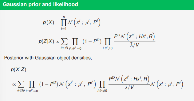
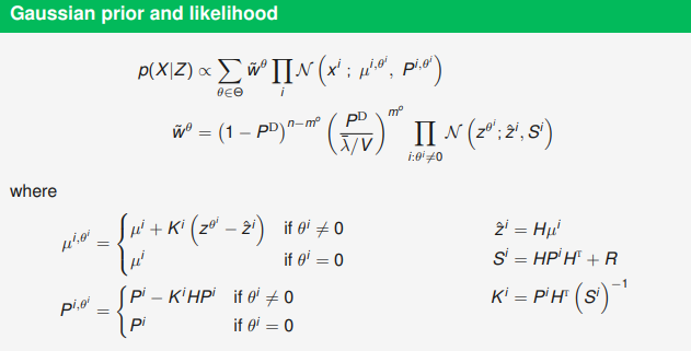
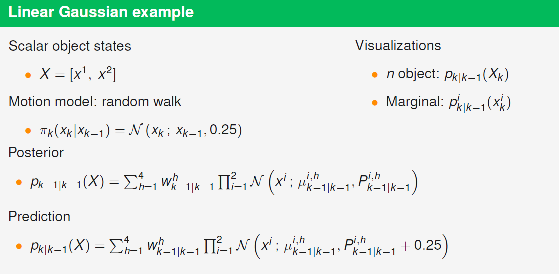
p ( X ∣ Z ) ∝ ∑ θ ∈ Θ ∏ i = 1 n w ~ θ i p i , θ i ( x i ) = ∑ θ ∈ Θ ∏ i ′ = 1 n w ~ θ i ′ ∏ i = 1 n p i , θ i ( x i ) = ∑ θ ∈ Θ w ~ θ ∏ i = 1 n p i , θ i ( x i ) = ∑ θ ∈ Θ w ~ θ p θ ( X ) \begin{aligned} p(X|Z) & \propto \sum_{\theta \in \Theta} \prod_{i=1}^n \tilde{w}^{\theta^i} p^{i,\theta^i}(x^i) = \sum_{\theta \in \Theta} \prod_{i'=1}^n \tilde{w}^{\theta^{i'}} \prod_{i=1}^n p^{i,\theta^i}(x^i) \\ & = \sum_{\theta \in \Theta} \tilde{w}^{\theta} \prod_{i=1}^n p^{i,\theta^i}(x^i) = \sum_{\theta \in \Theta} \tilde{w}^{\theta} p^{\theta}(X) \\ \; \end{aligned} p ( X ∣ Z ) ∝ θ ∈ Θ ∑ i = 1 ∏ n w ~ θ i p i , θ i ( x i ) = θ ∈ Θ ∑ i ′ = 1 ∏ n w ~ θ i ′ i = 1 ∏ n p i , θ i ( x i ) = θ ∈ Θ ∑ w ~ θ i = 1 ∏ n p i , θ i ( x i ) = θ ∈ Θ ∑ w ~ θ p θ ( X ) p ( X ∣ Z ) = ∑ θ ∈ Θ w θ p θ ( X ) p(X|Z) = \sum_{\theta \in \Theta} w^\theta p^\theta(X) p ( X ∣ Z ) = θ ∈ Θ ∑ w θ p θ ( X ) w θ = w ~ θ ∑ θ ′ w ~ θ ′ = ∏ i w ~ θ i ∑ θ ′ ∏ i ′ w ~ θ ′ i ′ w^\theta = \frac{\tilde{w}^{\theta}}{\sum_{\theta'} \tilde{w}^{\theta'}} = \frac{\prod_{i}\tilde{w}^{\theta^i}}{\sum_{\theta'}\prod_{i'}\tilde{w}^{\theta'^{i'}}} w θ = ∑ θ ′ w ~ θ ′ w ~ θ = ∑ θ ′ ∏ i ′ w ~ θ ′ i ′ ∏ i w ~ θ i 다음의 figure 2에서 Gaussian prior를 사용하는 예시를 볼 수 있다.
이제 다음과 같은 mixture prior를 가정하여 더 일반화된 식을 작성해보자.
p ( X ) = ∑ h P r ( h ) p ( X ∣ h ) w h p h ( X ) = ∑ h P r ( h ) p ( X ∣ h ) p(X) = \sum_h Pr(h)p(X|h)w^h p^h(X) = \sum_h Pr(h)p(X|h) p ( X ) = h ∑ P r ( h ) p ( X ∣ h ) w h p h ( X ) = h ∑ P r ( h ) p ( X ∣ h ) 위의 식을 사용하더라도 다음과 같이 posterior를 어떤 함수의 weigted sum으로 쓸 수 있다.
p ( X ∣ Z ) ∝ p ( Z ∣ X ) p ( X ) = [ ∑ θ ∈ Θ p ( Z , θ ∣ X ) ] [ ∑ h w h p h ( X ) ] = ∑ h ∑ θ ∈ Θ w h p ( Z , θ ∣ X ) p h ( X ) = ∑ h ∑ θ ∈ Θ w h w ~ θ ∣ h p ( Z , θ ∣ X ) p h ( X ) w ~ θ ∣ h = ∑ h ∑ θ ∈ Θ w ~ h , θ p h , θ ( X ) \begin{aligned} p(X|Z) & \propto p(Z|X)p(X) = \left[ \sum_{\theta \in \Theta } p(Z,\theta|X) \right]\left[ \sum_{h} w^h p^h(X) \right] \\ & = \sum_{h} \sum_{\theta \in \Theta} w^h p(Z,\theta|X) p^h(X) = \sum_{h} \sum_{\theta \in \Theta} w^h \tilde{w}^{\theta|h}\frac{p(Z,\theta|X) p^h(X)}{\tilde{w}^{\theta|h}} \\ & = \sum_{h} \sum_{\theta \in \Theta} \tilde{w}^{h,\theta}p^{h,\theta}(X) \end{aligned} p ( X ∣ Z ) ∝ p ( Z ∣ X ) p ( X ) = [ θ ∈ Θ ∑ p ( Z , θ ∣ X ) ] [ h ∑ w h p h ( X ) ] = h ∑ θ ∈ Θ ∑ w h p ( Z , θ ∣ X ) p h ( X ) = h ∑ θ ∈ Θ ∑ w h w ~ θ ∣ h w ~ θ ∣ h p ( Z , θ ∣ X ) p h ( X ) = h ∑ θ ∈ Θ ∑ w ~ h , θ p h , θ ( X ) 이때, w ~ θ ∣ h = ∫ p ( Z , θ ∣ X ) p h ( X ) d X = p ( Z , θ ∣ h ) \tilde{w}^{\theta|h} = \int{p(Z,\theta|X)p^h(X)dX}=p(Z,\theta|h) w ~ θ ∣ h = ∫ p ( Z , θ ∣ X ) p h ( X ) d X = p ( Z , θ ∣ h )
p ( X ∣ Z ) = ∑ h ∑ θ ∈ Θ w h , θ p h , θ ( X ) = ∑ h ∑ θ ∈ Θ P r ( h , θ ) p ( X ∣ h , θ ) p(X|Z) = \sum_{h} \sum_{\theta \in \Theta} w^{h,\theta}p^{h,\theta}(X) = \sum_{h} \sum_{\theta \in \Theta} Pr(h,\theta)p(X|h,\theta) p ( X ∣ Z ) = h ∑ θ ∈ Θ ∑ w h , θ p h , θ ( X ) = h ∑ θ ∈ Θ ∑ P r ( h , θ ) p ( X ∣ h , θ ) w h , θ = w ~ θ ∣ h w h ∑ h ∑ θ ∈ Θ w ~ θ ∣ h w h w^{h,\theta} = \frac{ \tilde{w}^{\theta|h} w^h }{\sum_{h} \sum_{\theta \in \Theta} \tilde{w}^{\theta|h} w^h} w h , θ = ∑ h ∑ θ ∈ Θ w ~ θ ∣ h w h w ~ θ ∣ h w h 여기에 time step k까지 추가하면 다음과 같이 쓸 수 있으며, 이러한 posterior를 통해 객체의 state에 대한 update를 수행할 수 있다.
p k ∣ k ( X k ) = p X k ∣ Z 1 : k ( X k ∣ Z 1 : k ) ∝ ∑ θ 1 : k w ~ k ∣ k θ 1 : k p k ∣ k θ 1 : k ( X k ) p_{k|k}(X_k)=p_{X_k | Z_{1:k}}(X_k | Z_{1:k}) \propto \sum_{\theta_{1:k}} \tilde{w}^{\theta_{1:k}}_{k|k} p^{\theta_{1:k}}_{k|k} (X_k) p k ∣ k ( X k ) = p X k ∣ Z 1 : k ( X k ∣ Z 1 : k ) ∝ θ 1 : k ∑ w ~ k ∣ k θ 1 : k p k ∣ k θ 1 : k ( X k ) w ~ k ∣ k θ 1 : k = ∏ i = 1 n ∏ t = 1 n w ~ θ t i ∣ θ 1 : t − 1 \tilde{w}^{\theta_{1:k}}_{k|k} = \prod_{i=1}^n \prod_{t=1}^n \tilde{w}^{\theta_{t}^i|\theta_{1:t-1}} w ~ k ∣ k θ 1 : k = i = 1 ∏ n t = 1 ∏ n w ~ θ t i ∣ θ 1 : t − 1 p k ∣ k θ 1 : k ( X k ) = ∏ i = 1 n p k ∣ k i , θ 1 : k i ( x k i ) p^{\theta_{1:k}}_{k|k} (X_k) = \prod_{i=1}^n p^{i,\theta^i_{1:k}}_{k|k} (x^i_k) p k ∣ k θ 1 : k ( X k ) = i = 1 ∏ n p k ∣ k i , θ 1 : k i ( x k i ) 이제 n개의 객체에 대한 prediction 과정을 살펴보자. Prediction을 위한 transition density는 다음과 같이 쓸 수 있다.
p k ( X k ∣ X k − 1 ) = p k ( x k 1 , x k 2 , ⋯ , x k i , ⋯ , x k n ) p_k(X_k|X_{k-1}) = p_k(x^1_k,x^2_k, \cdots, x^i_k, \cdots, x^n_k) p k ( X k ∣ X k − 1 ) = p k ( x k 1 , x k 2 , ⋯ , x k i , ⋯ , x k n ) 이때, 각 객체가 독립적으로 운동한다고 가정하면 다음과 같이 하나의 motion model을 사용하여 다음과 같이 간단하게 표현할 수 있다.
p k ( X k ∣ X k − 1 ) = ∏ i = 1 n π k ( x k i ∣ x k − 1 i ) p_k(X_k|X_{k-1}) = \prod_{i=1}^n \pi_k(x^i_k|x^i_{k-1}) p k ( X k ∣ X k − 1 ) = i = 1 ∏ n π k ( x k i ∣ x k − 1 i ) n개의 객체에 대한 Chapman-Kolmogorov prediction 식은 다음과 같다(위에서 사용된 notation처럼 p k ∣ k − 1 ( X k ) p_{k|k-1} (X_k) p k ∣ k − 1 ( X k ) p X k ∣ Z 1 : k − 1 ( X k ∣ Z 1 : k − 1 ) p_{X_k | Z_{1:k-1}}(X_k | Z_{1:k-1}) p X k ∣ Z 1 : k − 1 ( X k ∣ Z 1 : k − 1 )
p k ∣ k − 1 ( X k ) = ∫ p k ( X k ∣ X k − 1 ) p k − 1 ∣ k − 1 ( X k − 1 ) d X k − 1 p_{k|k-1} (X_k) = \int p_k(X_k|X_{k-1})p_{k-1|k-1}(X_{k-1}) d X_{k-1} p k ∣ k − 1 ( X k ) = ∫ p k ( X k ∣ X k − 1 ) p k − 1 ∣ k − 1 ( X k − 1 ) d X k − 1 Posterior p k − 1 ∣ k − 1 ( X k − 1 ) p_{k-1|k-1}(X_{k-1}) p k − 1 ∣ k − 1 ( X k − 1 )
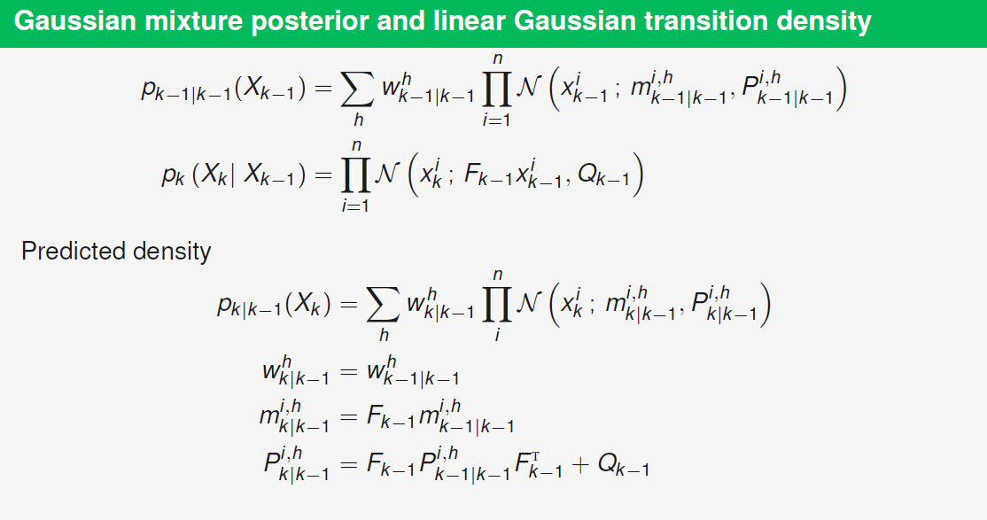
p k − 1 ∣ k − 1 ( X k − 1 ) = ∏ i = 1 n p k − 1 ∣ k − 1 i ( x k − 1 i ) p_{k-1|k-1}(X_{k-1}) = \prod_{i=1}^n p^i_{k-1|k-1}(x^i_{k-1}) p k − 1 ∣ k − 1 ( X k − 1 ) = i = 1 ∏ n p k − 1 ∣ k − 1 i ( x k − 1 i ) p k ∣ k − 1 ( X k ) = ∫ p k ( X k ∣ X k − 1 ) p k − 1 ∣ k − 1 ( X k − 1 ) d X k − 1 = ∫ ∫ ⋯ ∫ [ ∏ i = 1 n π k ( x k i ∣ x k − 1 i ) ] [ ∏ i ′ = 1 n p k − 1 ∣ k − 1 i ′ ( x k − 1 i ′ ) ] d x k − 1 1 ⋯ x k − 1 n = ∏ i = 1 n ∫ π k ( x k i ∣ x k − 1 i ) p k − 1 ∣ k − 1 i ( x k − 1 i ) d x k − 1 i = ∏ i = 1 n p k ∣ k − 1 i ( x k i ) \begin{aligned} p_{k|k-1} (X_k) & = \int p_k(X_k|X_{k-1}) p_{k-1|k-1}(X_{k-1}) d X_{k-1} \\ & = \int \int \cdots \int \left[ \prod_{i=1}^n \pi_k(x^i_k|x^i_{k-1}) \right] \left[ \prod_{i'=1}^n p^{i'}_{k-1|k-1}(x^{i'}_{k-1}) \right] d x^1_{k-1} \cdots x^n_{k-1} \\ & = \prod_{i=1}^n \int \pi_k(x^i_k|x^i_{k-1}) p^{i}_{k-1|k-1}(x^{i}_{k-1}) d x^i_{k-1} = \prod_{i=1}^n p^i_{k|k-1} (x^i_k) \end{aligned} p k ∣ k − 1 ( X k ) = ∫ p k ( X k ∣ X k − 1 ) p k − 1 ∣ k − 1 ( X k − 1 ) d X k − 1 = ∫ ∫ ⋯ ∫ [ i = 1 ∏ n π k ( x k i ∣ x k − 1 i ) ] [ i ′ = 1 ∏ n p k − 1 ∣ k − 1 i ′ ( x k − 1 i ′ ) ] d x k − 1 1 ⋯ x k − 1 n = i = 1 ∏ n ∫ π k ( x k i ∣ x k − 1 i ) p k − 1 ∣ k − 1 i ( x k − 1 i ) d x k − 1 i = i = 1 ∏ n p k ∣ k − 1 i ( x k i ) Posterior p k − 1 ∣ k − 1 ( X k − 1 ) p_{k-1|k-1}(X_{k-1}) p k − 1 ∣ k − 1 ( X k − 1 )
p k − 1 ∣ k − 1 ( X k − 1 ) = ∑ h w k − 1 ∣ k − 1 h p k − 1 ∣ k − 1 ( X k − 1 ) p_{k-1|k-1}(X_{k-1}) = \sum_{h} w^h_{k-1|k-1} p_{k-1|k-1}(X_{k-1}) p k − 1 ∣ k − 1 ( X k − 1 ) = h ∑ w k − 1 ∣ k − 1 h p k − 1 ∣ k − 1 ( X k − 1 ) p k ∣ k − 1 ( X k ) = ∫ p k ( X k ∣ X k − 1 ) p k − 1 ∣ k − 1 ( X k − 1 ) d X k − 1 = ∫ p k ( X k ∣ X k − 1 ) [ ∑ h w k − 1 ∣ k − 1 h p k − 1 ∣ k − 1 ( X k − 1 ) ] d X = ∑ h w k − 1 ∣ k − 1 h ∫ p k ( X k ∣ X k − 1 ) p k − 1 ∣ k − 1 ( X k − 1 ) d X = ∑ h w k − 1 ∣ k − 1 h p k ∣ k − 1 h ( X k ) \begin{aligned} p_{k|k-1} (X_k) & = \int p_k(X_k|X_{k-1}) p_{k-1|k-1}(X_{k-1}) d X_{k-1} \\ & = \int p_k(X_k|X_{k-1}) \left[ \sum_{h} w^h_{k-1|k-1} p_{k-1|k-1}(X_{k-1}) \right] dX \\ & = \sum_{h} w^h_{k-1|k-1} \int p_k(X_k|X_{k-1}) p_{k-1|k-1}(X_{k-1}) dX = \sum_{h} w^h_{k-1|k-1} p^h_{k|k-1} (X_k) \end{aligned} p k ∣ k − 1 ( X k ) = ∫ p k ( X k ∣ X k − 1 ) p k − 1 ∣ k − 1 ( X k − 1 ) d X k − 1 = ∫ p k ( X k ∣ X k − 1 ) [ h ∑ w k − 1 ∣ k − 1 h p k − 1 ∣ k − 1 ( X k − 1 ) ] d X = h ∑ w k − 1 ∣ k − 1 h ∫ p k ( X k ∣ X k − 1 ) p k − 1 ∣ k − 1 ( X k − 1 ) d X = h ∑ w k − 1 ∣ k − 1 h p k ∣ k − 1 h ( X k ) 다만, 각 객체가 독립적으로 운동한다는 가정은 상황에 따라 틀린 가정이 될 수 있음에 유의하여야 한다.
4. Data Association as an Optimization Problem
Mixture posterior의 업데이트 식 등에서 모든 data association에 대한 summation이 요구되는데 한정된 컴퓨팅 자원 상에서 이렇게 모든 data association에 대해 연산을 하는 것은 매우 힘들다. 따라서 우리는 근사를 통해 불필요한 연산을 줄이는 작업이 필요하며, 이를 해결하기 위한 대표적인 아이디어는 큰 weight w ~ θ k ∣ h \tilde{w}^{\theta_k|h} w ~ θ k ∣ h θ k ∈ Θ ~ k \theta_k \in \tilde{\Theta}_k θ k ∈ Θ ~ k ∣ Θ ~ k ∣ ≪ ∣ Θ k ∣ |\tilde{\Theta}_k| \ll |\Theta_k| ∣ Θ ~ k ∣ ≪ ∣ Θ k ∣ Θ ~ k \tilde{\Theta}_k Θ ~ k θ k \theta_k θ k
이를 수행하기 위하여 data asscoation 문제를 최적화(optimization) 문제로 생각하여 풀게 된다. 비슷한 문제로 작업할당 문제가 있는데, 여러 면의 worker에게 각각의 작업을 할당하며, 이때 발생하는 비용이 최소화되는 할당 방법을 찾는 문제이다. 이 문제를 matrix로 표현하면 다음과 같이 cost matrix와 assignment matrix로 표현할 수 있다.
C o s t M a t r i x : L = ( 5 8 7 8 12 7 4 8 5 ) \begin{aligned} Cost \; & Matrix : \\ & L = \begin{pmatrix} 5 & 8 & 7\\ 8 & 12 & 7 \\ 4 & 8& 5 \end{pmatrix} \end{aligned} C o s t M a t r i x : L = ⎝ ⎜ ⎛ 5 8 4 8 1 2 8 7 7 5 ⎠ ⎟ ⎞ A s s i g n m e n t M a t r i x : A = ( 0 1 0 0 0 1 1 0 0 ) \begin{aligned} Assignment \; & Matrix : \\ & A = \begin{pmatrix} 0 & 1 & 0\\ 0 & 0 & 1 \\ 1 & 0 & 0 \end{pmatrix} \end{aligned} A s s i g n m e n t M a t r i x : A = ⎝ ⎜ ⎛ 0 0 1 1 0 0 0 1 0 ⎠ ⎟ ⎞ 여기서 cost matrix는 각 worker가 해당 작업을 수행했을 때 발생하는 비용을 포함하는 matrix이며, assignment matrix는 어떤 worker가 어떤 작업을 맡고 있는 지를 표현한다(worker w i w^i w i t j t^j t j A i , j = 1 A^{i, j}=1 A i , j = 1 A i , j = 0 A^{i, j}=0 A i , j = 0
위와 같이 matrix가 주어졌을 때, 발생하는 총 비용은 다음과 같이 구할 수 있다.
C o s t = ∑ i ∑ j A i , j L i , j = t r ( A T L ) Cost = \sum_i \sum_j A^{i, j}L^{i, j} = tr(A^TL) C o s t = i ∑ j ∑ A i , j L i , j = t r ( A T L ) 이제 data association을 위와 같은 형태로 적용해보자. 주어진 h h h θ ∗ ∈ Θ \theta^* \in \Theta θ ∗ ∈ Θ
w ~ θ ∗ ∣ h ≥ w ~ θ ∣ h , ∀ θ ∈ Θ \tilde{w}^{\theta^* | h} \ge \tilde{w}^{\theta | h}, \forall \theta \in \Theta w ~ θ ∗ ∣ h ≥ w ~ θ ∣ h , ∀ θ ∈ Θ 따라서 optimal data association을 찾기 위한 optimization 문제는 다음과 같이 쓸 수 있다.
θ ∗ = a r g m a x θ ∈ Θ w ~ θ ∣ h = a r g m a x θ ∈ Θ ∏ i = 1 n w ~ θ i ∣ h \theta^* = \underset{\theta \in \Theta}{argmax} \; \tilde{w}^{\theta | h} = \underset{\theta \in \Theta}{argmax} \; \prod_{i=1}^n \tilde{w}^{\theta^i | h} θ ∗ = θ ∈ Θ a r g ma x w ~ θ ∣ h = θ ∈ Θ a r g ma x i = 1 ∏ n w ~ θ i ∣ h 여기에 단조 증가 함수인 log를 적용하여도 마찬가지로 maximization 문제로 유지된다.
θ ∗ = a r g m a x θ ∈ Θ log ( ∏ i = 1 n w ~ θ i ∣ h ) = a r g m a x θ ∈ Θ ∑ i = 1 n log ( w ~ θ i ∣ h ) \theta^* = \underset{\theta \in \Theta}{argmax} \; \log{\left( \prod_{i=1}^n \tilde{w}^{\theta^i | h} \right)} = \underset{\theta \in \Theta}{argmax} \; \sum_{i=1}^n \log (\tilde{w}^{\theta^i | h}) θ ∗ = θ ∈ Θ a r g ma x log ( i = 1 ∏ n w ~ θ i ∣ h ) = θ ∈ Θ a r g ma x i = 1 ∑ n log ( w ~ θ i ∣ h ) 여기에 -1을 곱하여 minimization 문제로 치환한다.
θ ∗ = a r g m i n θ ∈ Θ ∑ i = 1 n − log ( w ~ θ i ∣ h ) \theta^* = \underset{\theta \in \Theta}{argmin} \; \sum_{i=1}^n -\log (\tilde{w}^{\theta^i | h}) θ ∗ = θ ∈ Θ a r g min i = 1 ∑ n − log ( w ~ θ i ∣ h ) 이렇게 치환된 문제는 다음과 같이 비용을 최소화하는 opimization 문제와 같으며, 해당 최적화 문제의 해법을 적용할 수 있다.
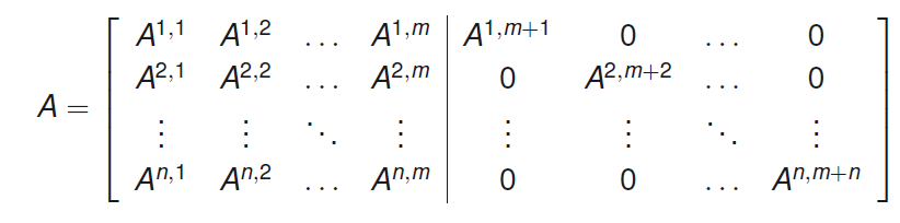
A ∗ = a r g m i n A t r ( A T L ) A^* = \underset{A}{argmin} \; tr(A^TL) A ∗ = A a r g min t r ( A T L ) Data association 문제의 assignment matrix는 n × ( m + n ) n \times (m+n) n × ( m + n ) θ i = j \theta^i = j θ i = j A i , j = 1 A^{i,j}=1 A i , j = 1 θ i = 0 \theta^i = 0 θ i = 0 A i , m + i = 1 A^{i,m+i}=1 A i , m + i = 1 n × m n \times m n × m n × n n \times n n × n
이제 cost matrix를 살펴보자. 위에서 전개한 식에 따르면 주어진 hypothesis h에 대해서 un-normalized association weight는 다음과 같다.
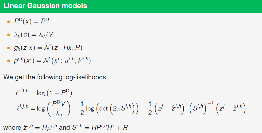
w ~ θ i ∣ h = { ∫ ( 1 − P D ( x i ) ) p i , h ( x i ) d x i i f θ i = 0 ∫ P D ( x i ) g ( z θ i ∣ x i ) λ c ( z θ i ) p i , h ( x i ) d x i i f θ i ≠ 0 \tilde{w}^{\theta^i|h} = \begin{cases} \int (1-P^D(x^i))p^{i,h}(x^i) dx^i \;\;\;\;\;\; if \; \theta^i = 0 \\ \int{\frac{P^D(x^i)g(z^{\theta^i}|x^i)}{\lambda_c(z^{\theta^i})}p^{i,h}(x^i)} dx^i \;\;\;\;\;\;\; if \; \theta^i \ne 0 \end{cases} w ~ θ i ∣ h = ⎩ ⎪ ⎨ ⎪ ⎧ ∫ ( 1 − P D ( x i ) ) p i , h ( x i ) d x i i f θ i = 0 ∫ λ c ( z θ i ) P D ( x i ) g ( z θ i ∣ x i ) p i , h ( x i ) d x i i f θ i = 0 이 식에 log를 적용하여 log-likelihood를 다음과 같이 구할 수 있다.
l i , 0 , h = log ( ∫ ( 1 − p D ( x i ) ) p i , h ( x i ) d x i ) l^{i,0,h}=\log \left( \int (1-p^D(x^i))p^{i,h}(x^i)dx^i \right) l i , 0 , h = log ( ∫ ( 1 − p D ( x i ) ) p i , h ( x i ) d x i ) 검출되었을 때, 즉 x i x^i x i z i z^i z i
l i , j , h = log ( ∫ P D ( x i ) g ( z j ∣ x i ) λ c ( z j ) p i , h ( x i ) d x i ) l^{i,j,h}=\log \left( \int{\frac{P^D(x^i)g(z^{j}|x^i)}{\lambda_c(z^{j})}p^{i,h}(x^i)} dx^i \right) l i , j , h = log ( ∫ λ c ( z j ) P D ( x i ) g ( z j ∣ x i ) p i , h ( x i ) d x i )
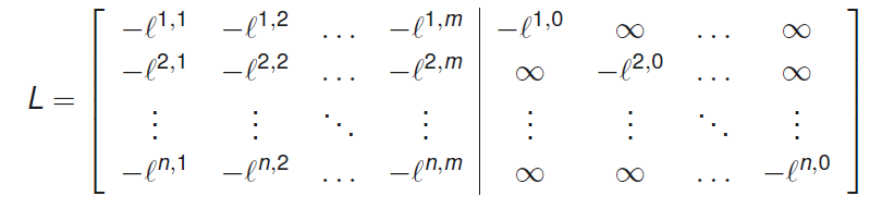
이제 위와 같이 계산된 negative log-weight의 합을 최소화 해야하는데, 전체 cost는 다음과 같이 assignment matrix를 통해 표현될 수 있다.
∑ i = 1 n − log ( w ~ θ i ∣ h ) = ∑ i = 1 n ∑ j = 1 m A i , j ( − l i , j , h ) + ∑ i ′ = 1 n A i ′ , m + i ′ ( − l i , 0 , h ) \sum_{i=1}^n -\log (\tilde{w}^{\theta^i | h}) = \sum_{i=1}^n \sum_{j=1}^m A^{i,j} (-l^{i,j,h}) + \sum_{i'=1}^n A^{i',m+i'} (-l^{i,0,h}) i = 1 ∑ n − log ( w ~ θ i ∣ h ) = i = 1 ∑ n j = 1 ∑ m A i , j ( − l i , j , h ) + i ′ = 1 ∑ n A i ′ , m + i ′ ( − l i , 0 , h ) 이제 적당한 형태의 cost matrix L L L L L L n × m n \times m n × m n × n n \times n n × n t r ( A T L h ) tr(A^TL^h) t r ( A T L h ) w ~ θ ∣ h = e x p ( − t r ( A T L h ) ) \tilde{w}^{\theta | h} = exp(-tr(A^TL^h)) w ~ θ ∣ h = e x p ( − t r ( A T L h ) ) θ \theta θ
∑ i = 1 n − log ( w ~ θ i ∣ h ) = ∑ i = 1 n ∑ j = 1 m + n A i , j L i , j , h = t r ( A T L h ) \sum_{i=1}^n -\log (\tilde{w}^{\theta^i | h}) = \sum_{i=1}^n \sum_{j=1}^{m+n} A^{i,j} L^{i,j,h} = tr(A^TL^h) i = 1 ∑ n − log ( w ~ θ i ∣ h ) = i = 1 ∑ n j = 1 ∑ m + n A i , j L i , j , h = t r ( A T L h )
해결해야하는 전체적 최적화 문제는 다음과 같이 요약할 수 있고, 이러한 문제를 풀기위한 방법으로 best solution A ∗ A^* A ∗
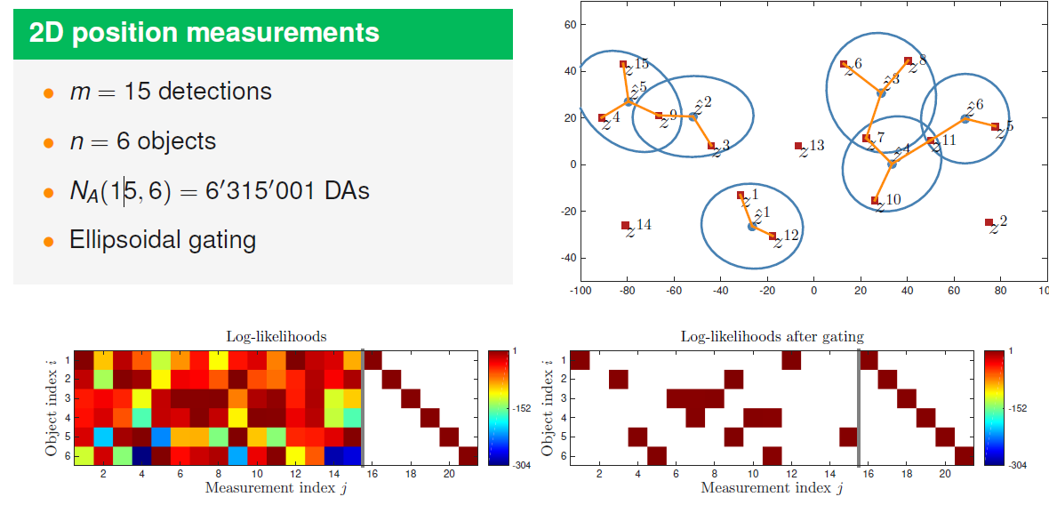
m i n i m i z e t r ( A t L ) s u b j e c t t o A i , j ∈ { 0 , 1 } , i , j ∈ { 1 , ⋯ , n } × { 1 , ⋯ , n + m } ∑ j = 1 n + m A i , j = 1 , i ∈ { 1 , ⋯ , n } ∑ j = 1 n A i , j ∈ { 0 , 1 } , j ∈ { 1 , ⋯ , n + m } \begin{aligned} & minimize \;\;\;\;\; tr(A^tL) \\ & subject \; to \;\;\;\;\; A^{i,j} \in \{0, 1\}, \;\;\;\;\;\;\;\;\;\;\;\;\; i,j \in \{1, \cdots, n\} \times \{1, \cdots, n+m\} \\ & \;\;\;\;\;\;\;\;\;\;\;\;\;\;\;\;\;\;\;\; \sum^{n+m}_{j=1} A^{i,j} = 1, \;\;\;\;\;\;\;\;\;\;\;\;\; i \in \{1, \cdots, n\} \\ & \;\;\;\;\;\;\;\;\;\;\;\;\;\;\;\;\;\;\;\; \sum^{n}_{j=1} A^{i,j} \in \{0,1\}, \;\;\;\;\;\;\; j \in \{1, \cdots, n+m\} \end{aligned} m i n i m i z e t r ( A t L ) s u b j e c t t o A i , j ∈ { 0 , 1 } , i , j ∈ { 1 , ⋯ , n } × { 1 , ⋯ , n + m } j = 1 ∑ n + m A i , j = 1 , i ∈ { 1 , ⋯ , n } j = 1 ∑ n A i , j ∈ { 0 , 1 } , j ∈ { 1 , ⋯ , n + m } 또한 SOT gating을 통해 연산량을 줄일 수 있는 데 gating에서는 특정 distance 함수를 정의하고, 해당 distance가 일정 threshold 이상으로 증가하면 해당 association을 무시한다. 예를 들어 distance 함수는 다음과 같이 ellipsoidal gating distance를 정의할 수 있으며, 이는 figure 5의 log-likelihood에도 나타난다.
d i , j , h 2 = ( z k j − z ^ k ∣ k − 1 i , h ) T ( S k i , h ) − 1 ( z k j − z ^ k ∣ k − 1 i , h ) d_{i,j,h}^2 = (z^{j}_k - \hat{z}^{i,h}_{k|k-1})^T (S^{i,h}_{k})^{-1}(z^{j}_k - \hat{z}^{i,h}_{k|k-1}) d i , j , h 2 = ( z k j − z ^ k ∣ k − 1 i , h ) T ( S k i , h ) − 1 ( z k j − z ^ k ∣ k − 1 i , h ) 해당 distance가 커지면 log-likelihood는 감소하고, threshold G 이상으로 증가하면 해당 association l i , j , h = − ∞ l^{i,j,h}=-\infin l i , j , h = − ∞
또한 뒤에서는 연산량을 줄이기 위한 여러 tracking algorithm을 소개한다.