3D 그래프를 그리기 위한 라이브러리
불러오기
from mpl_toolkits.mplot3d import Axes3D
그래프
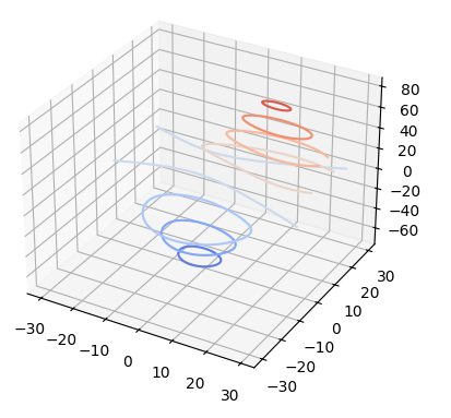
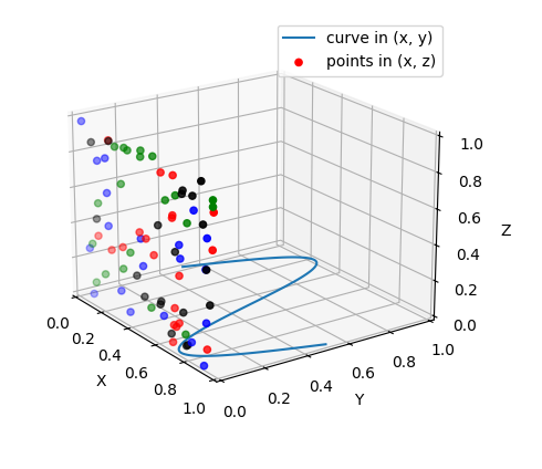
1) Line plots
: plot 2D or 3D data
Axes3D.plot(xs, ys, *args, zdir='z', **kwargs)
- xs : 1D array-like
- ys : 1D array-like
- zs : float or 1D array-like
- zdir : {'x', 'y', 'z'}, default: 'z'
When plotting 2D data, the direction to use as z.
2) Scatter plots
Axes3D.scatter(xs, ys, zs=0, zdir='z', s=20, c=None, depthshade=True, *args, data=None, **kwargs)
3) Wireframe plots
Axes3D.plot_wireframe(X, Y, Z, **kwargs)
-
X, Y, Z : 2D arrays
-
rcount, ccountint (Defaults to 50)
Maximum number of samples used in each direction. If the input data is larger, it will be downsampled (by slicing) to these numbers of points. Setting a count to zero causes the data to be not sampled in the corresponding direction, producing a 3D line plot rather than a wireframe plot. -
rstride, cstrideint
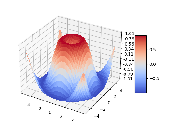
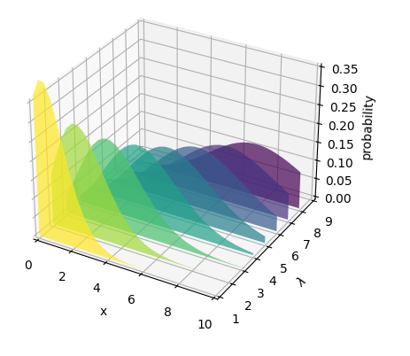
4) Surface plots
Axes3D.plot_surface(X, Y, Z, *, norm=None, vmin=None, vmax=None, lightsource=None, **kwargs)
- X, Y, Z : 2D arrays
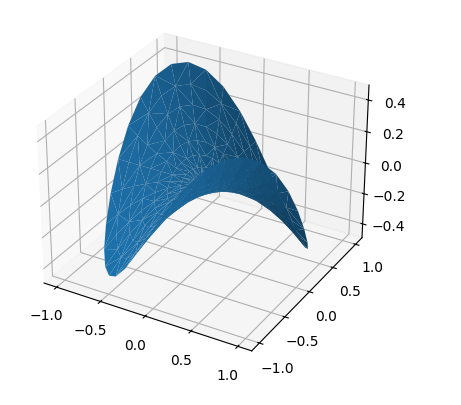
5) Tri-Surface plots
Axes3D.plot_trisurf(*args, color=None, norm=None, vmin=None, vmax=None, lightsource=None, **kwargs)
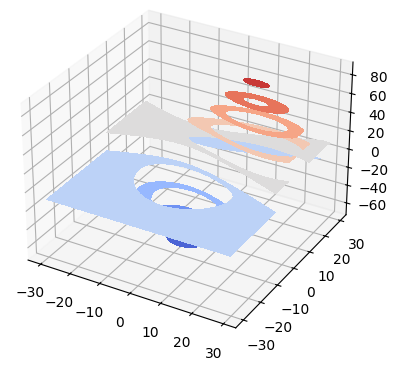
6) Contour plots
Axes3D.contour(X, Y, Z, *args, extend3d=False, stride=5, zdir='z', offset=None, data=None, **kwargs)
7) Filled contour plots
Axes3D.contourf(X, Y, Z, *args, zdir='z', offset=None, data=None, **kwargs)
8) polygon plots
Axes3D.add_collection3d(col, zs=0, zdir='z')
2D collection types are converted to a 3D version by modifying the object and adding z coordinate information.
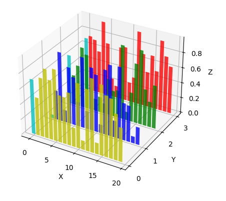
9) bar plots
Axes3D.bar(left, height, zs=0, zdir='z', *args, data=None, **kwargs)
-
left : 1D array-like
The x coordinates of the left sides of the bars. -
height : 1D array-like
The height of the bars. -
zs : float or 1D array-like
Z coordinate of bars; if a single value is specified, it will be used for all bars. -
zdir : {'x', 'y', 'z'}, default: 'z'
When plotting 2D data, the direction to use as z ('x', 'y' or 'z'). -
data : indexable object, optional
9) Quiver
Axes3D.quiver(X, Y, Z, U, V, W, *, length=1, arrow_length_ratio=0.3, pivot='tail', normalize=False, data=None, **kwargs)

10) 2D plot in 3D
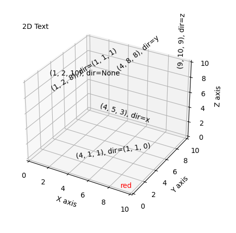
11) Text
Axes3D.text(x, y, z, s, zdir=None, **kwargs)
-
x, y, z : float
The position to place the text. -
s : str(The text)
-
zdir : {'x', 'y', 'z', 3-tuple}, optional
The direction to be used as the z-direction. Default: 'z'. See get_dir_vector for a description of the values.
필사연습
from mpl_toolkits.mplot3d import Axes3D
import matplotlib.pyplot as plt
from matplotlib import cm
import numpy as np
fig=plt.figure() #그래프 객체 생성
ax=fig.add_subplot(111, projection='3d') #Axes3D 축을 fig에 추가
# 111은 그려질 서브플롯의 위치로 1,1,1 과 동일 (최대 10 정수 사용가능)
# projection='3d' 객체가 그래프에 투용될 방법 ( None, 'mollweide', 'polar', 'rectilinear', str 등)
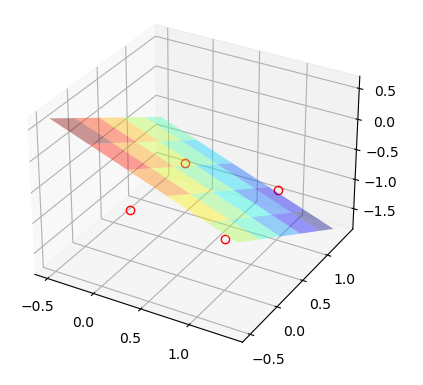
x = [0, 0, 1, 1]
y = [0, 1, 0, 1]
z = [-1, -1, -1, -1]
#좌표(x, y, z) = (0, 0, -1), (0, 1, -1), (1, 0, -1), (1, 1, -1)
X = np.arange(-0.5, 1.5, 0.1)
Y = np.arange(-0.5, 1.5, 0.1) # -0.5에서 1.5까지 0.1을 간격으로 array를 생성한 것을 각각 X, Y에 대입
X, Y = np.meshgrid(X, Y)
Z = (float(-5/7) * Y) + (float(-4/7) *X) #가중치 [0.14 0.1 0.08]를 0.14Z + 0.1X + 0.08Y = 0 평면의 방정식으로 바꾼 것을 Z에 대한 식으로 정리
ax.plot(x, y, z, linestyle='none', marker='o', mfc='none', markeredgecolor='red')
ax.plot_surface(X,Y,Z, rstride=4, cstride=4, alpha=0.4, cmap=cm.jet) #rstride, stride는 각각 색의 변화율을 설정, 기본값 1, 숫자가 커질수록 변화 커짐
plt.show()