Deep Generative Modeling

supervised vs unsupervised learning

Supervised Learning

Data : $(x, y)$
$x$ is data, $y$ is label

Goal : Learn function to map ($x -> y$)

Examples : classification, regression, object detection, semantic segmentation

Unsupervised Learning

Data : $x$
$x$ is data, no labels!

Goal : Learn some hidden or underlying structure of the data

Examples : Clustering, feature or dimensionality reduction, deep generative modeling

unsupervised learning captures the idea of deep generative modeling.

Generative modeling

Goal : Take as input training samples from some distribution and learn a model that represents that distribution

The generative modeling has a two forms : density estimation / sample generation

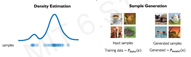
density estimation : the goal is to train a model that learns a underlying probability distribution that describes where the data came from

smaple generation : similar to density estimation, but focus more on generaing new instances. The model learns a underlying probability distribution, but then use that model to sample from it and generate new instances.

underlying question : How can we learn $P_{model}(x)$ similar to $P_{data}(x)$?

Why generative models?

The generative models have ability to uncover the underlying features in a dataset and encode it in an efficient way. For example, if we are considering the problem of facial detection and given many different faces.

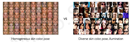
The data has so many variants(head, clothing, glasses, skin tone, hair). Additionally, the data may be very biased towards particular features. The generative model figures out underlying features in automatic way without any labeling. It uncovers what features may be overrepresented or underrpresented.

Another powerful example of generative model is outlier detection(identifying rare events).

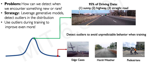
In self-driving problem, we want to make car can be able to handle all the possible scenarios including edge cases(deer or airplane coming in front of the car). We can apply the idea of density estimation to be able to identify rare events.

A broad class of generative models: latent variable models

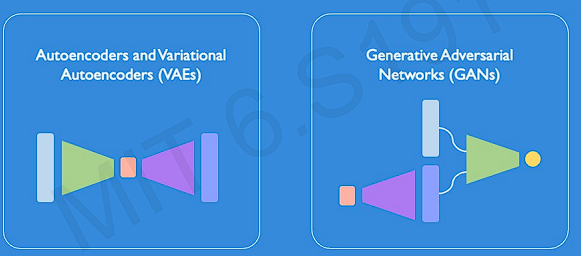
The latent variable models have two typical subtype models : VAEs and GANs

What is latent variable?

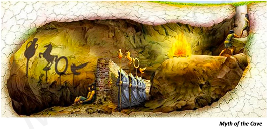
In the figure, the prisoners can only observe shadows of objects on the wall. They can measure the shadows and give names beacuse the shadows are reality to them. But they are unable to directly see the underlying objects the true factors themselves that are casting those shadows.

These shadows are like latent variables in machin learning. The variables are not directly observable, but they are the true underlying factors or explanatory factors. This gets out the models goal that the model can learn these hidden features even when we are given only observation data.

Autoencoders

A very simple generative model.

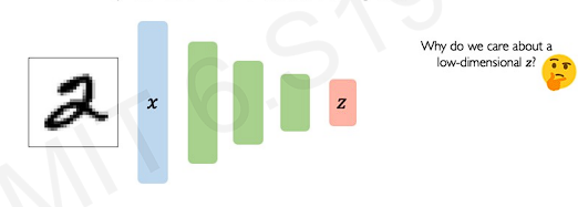
First it takes the raw input data, and pass it through a series of neural network layers. the output of this first step is low dimensional latent space($z$). The output is an encoded representation of those underlying features.

Then why do we mainly care about latent space? The first output(latent spcae) is a very efficient compact encoding of the rich high-dimensional data. Shortly, we can compress data into this small feature representation. It captures compactness and richness!

How do we actually train the network to learn this latent variable vector?
What the auto encoder does it is builds a way to decode this latent variable back upt to the original space.

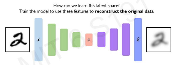
As we can see, 'encoder' learns mapping from $x$ to a low-dimensional space $z$, and 'decoder' learns mapping back from latent space z to reconstructed observation $\hat{x}$. The reconstructed output is an imperfection reconstruction.

To train this networks, all we have to do is compare the outputted reconstruction and the original input data and make these as similar as possible.

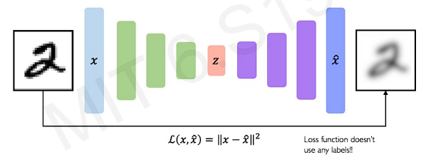
We can compare the pixel wise difference between the input data and the reconstructed output. The thing is, we don't need any labels for loss function. We just need the original input data $x$ and the reconstructed output $\hat{x}$.

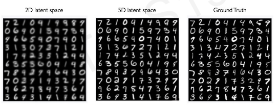
Autoencoding is a form of compression. So the lower dimensionality of the latent space has the less good reconstruction. Smaller(low-dimension) latent space will also force a larger training bottleneck. In contrast, The higher dimensionality has the less efficient encoding.

Variational Autoencoders(VAEs)

The traditional autoencoders are deterministic. It means that once the weights or activations are determined, the model gets the same exact outputs with the same inputs. In contrast, VAEs introduce a element of randomness a probabilistic twist on this idea of autoencoding. This make the model generates new images.

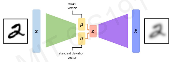
VAEs replace single deterministic layer with a random sampling operation.
We define mean and standard deviation that captures a probability distribution. Those mean and deviation parameterize the probability distributions of the latent variables.

Let's focus on how the model train the data.

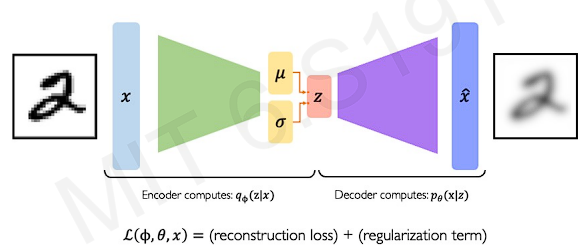
Since we've eliminated deterministic parameters, we now have these encoders and decoders as probabilistic. The encoders compute a probability distribution of $z$ given input data $x$, and the decoders do inverse. We define $\phi$ and $\theta$ to define network weights for encoding and decoding components.

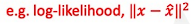
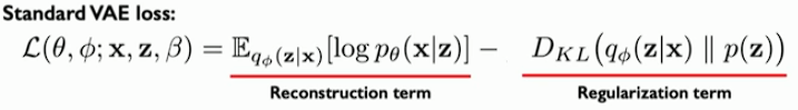
Then, we define a loss function(see the figure). We want to optimize the network weights($\phi$ and $\theta$) w.r.t the data by this function. The first term of the equation is the reconstruction loss where the goal is to capture difference between our input data and the reconstructed output. The second term is called regularization term. It is referred to as a vae loss.

We define reconstruction loss just similar to autoencoder.

And we define regularization term.

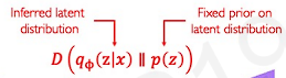
To define the regularization loss(about weight loss), we use prior latent distribution(denoted as $p(z)$) to constrain inferred latent distribution, so that it behaves nicely. The prior latent distribution is some initial hypothesis or guess about what that latent variable space may look like. This prior latent distribution enforces a latent space to follow it.
$D$ is regularization term that computes the distance between latent space and prior hypothesis.

The common choice of prior hypothesis is Normal Gaussian Distribution.
$p(z) = N(\mu = 0, \sigma^2 = 1)$

• This encourages encodings to distribute encodings evenly around the center of the latent space
  ->distributing the encoding smoothly so that we don't get too much divergence.
• This penalizes the network when it tries to "cheat" by clustering points in specific regions(i.e, by memorizing the data)

The mathematical term($D$) computes the distance divergence between prior and latent. This is called as KL-divergence.

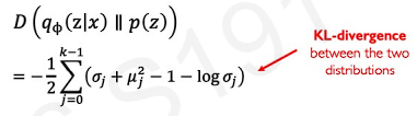
The important thing is KL-divergence trys to smooth the probability distribution.

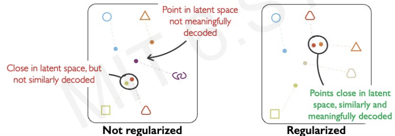
What is the intuition behind this regularization operation?
We do regularizing to achieve continuity and completeness.
The continuity is that if there are points that are close in latent space, we should recover 2 reconstructions that are similar in content.
The completeness is that we don't want the latent space has a gap. Since we decode and sample from the latent space, so the space has to be smooth and connected.

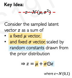
Problem : We cannot backpropagate gradients through sampling layers!
This is because backpropagation requires completely deterministic nodes and layers.

To apply backpropagation to train algorithm, key idea is reparametrizing the sampling layer. We rebuild the vector z(as a latent variable) with fixed vector, and fixed distribution(normal distribution).

We can understand how the backpropagation is possible by the following figure.

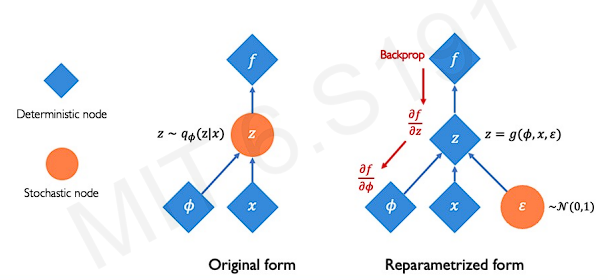
It is possible to update deterministic parameters($\phi, x$)

Let's apply it to real problem.

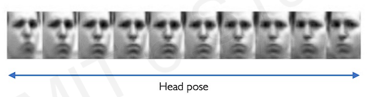
When we impose the prior distribution, it allows a single latent variable slowly perturb(increase or decrease) while keeping other single latent variables fixed. We can run the decoder of the vae evry time. And an individual latent variable is capturing meaningful information during we reconstruct the image every time. As we can see the example, the head is shifting by perturbing a sinlge latent variable.
The network becomes able to learn the features by perturbing them individually.

We want the most compact and richest form of represenation of the image, we consider one single latent variable with others simultaneously. We want to find the latent features that are as uncorrelated with others as possible(disentangled!).

We can enforces the network to get compact form from latent variables.

What we really need to know in this equation is that the equation has two terms for two loss. The more important thing is beta VAEs.

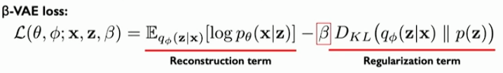
The parameter beta is weight constant.
If the $\beta$ is greater than 1, it constrains latent bottleneck, encourages efficient latent encoding. This provides disentanglement.

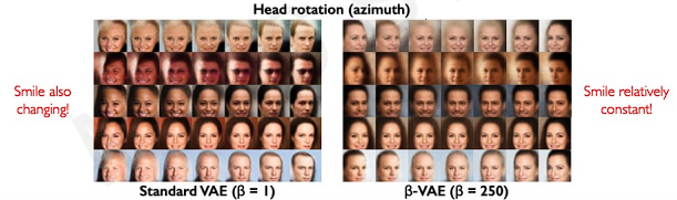
The example shows that when we rotate a head in the image, smile also changes if $\beta = 1$, but we can only rotate the head if $\beta > 1$.

VAE Summary

1. Compress representation of world to something we can use to learn.
2. Reconstruction allows for unsupervised learning(no labels!)
3. Reparameterization trick to train end-to-end
4. Interpret hidden latent variables using perturbation.
5. Generating new examples.

Generative Adversarial Networks(GANs).

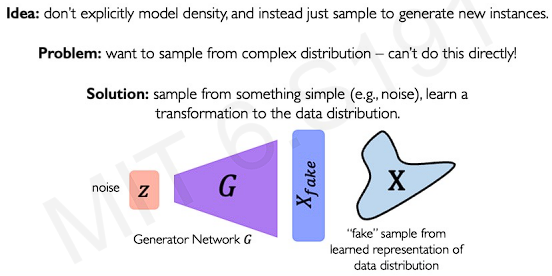
The goal of GANs is that we care more about how well we generate new instances which are similar to the existing data. However, the distribution from the original data is extremely difficult.

Then, how about generate synthetic examples from complete random noise? This is the goal of GANs(from noise, we want to generate examples as close to the real deal as possible.)

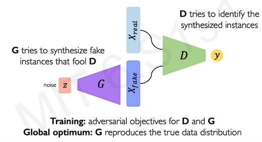
The key idea is to interface two neural networks. One is a generator and one is a discriminator. This two networks compet with each other.

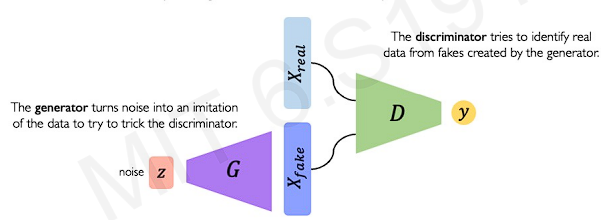
The generator trys to generate samples as close to real as possible. The discriminator takes real data and generated samples to learn a classification distinguishing real from fake.

The following figure tells the intuition behind GANs.

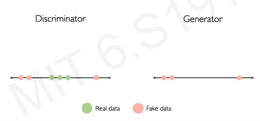
Let's start with 1-D line. The generator will generate fake data on the line. Then, the discriminator sees these points with some real data. Before it is trained. It might not well distinguish which one is real.

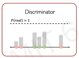
After training, it starts increasing the probability for those real data until the discriminator reaches the ability of perfect classification($p$($real$) = 1).
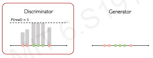
Now, we go back to generator. The generator sees where the real data lie on the line. Then, it is forced to start moving its generated fake data closer and closer to the real data. Then, the discriminator repeats the training(same process) for perfect classification.

This process repeats until the fake data is almost following the distribution of the real data.

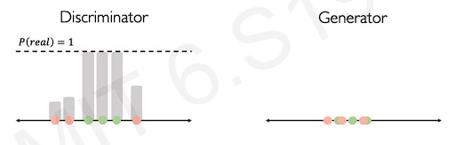
After the fake data is really close to the real data, the points become very hard to distinguish between what is real or what is fake.

This figure explains well of training GANs.

The dicriminator can be defined mathematically in terms of a loss objective.

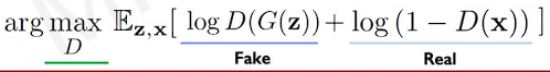
The equation tells to maximize probability of the real data.

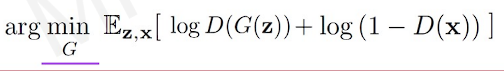
With the generator, we have same equation, but the goal is different(the goal is to minimize distances between fake and real).

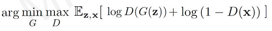
We can put this terms together in one equation.

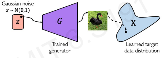
After training, we can use generator to create new data that has never been seen before(but still mimics the true data distribution).

What GANs are doing is to learn a function that transforms the distribution of random noise to some target. This is a function that maps to target space from noise space.


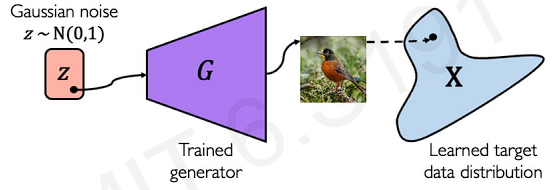
After mapping two real images, what we can do is interpolate and traverse between trajectories in the noise space. This trajectories are also mapped in the target space.