Computer Vision
To discover from images what is presnt in the world, where things are, what actions are taking place, to predict and anticipate events in the world.
The rise and impact of computer vision
Robotics / Mobile computing / Biology & Medicine / Autonomous driving / Facial Detection & Recognition / Accessibility
What Computers "See"
Images are numbers for computers. Image are made up of pixels. And the pixels are numbers. Therefore, we can represent image to 2D matrix.
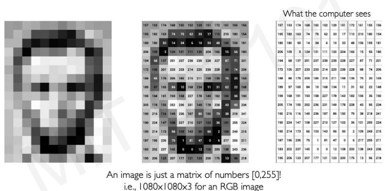
A color image has 3D matrix -> for colors(red or green or blue)
We have two task in computer vision
- Regression : output variable takes continuous value
- Classification : output variable takes class label. It can produce probability of belonging to a particular class
example for classification:
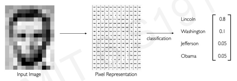
the goal of model in this example is to output a probability score. The model needs the ability to be able to tell what is unique about this particular image versus other images. Another way to think of this process is to figure out patterns(or characteristic) in our data.
Classification is simply done by detecting all of different pattern in images.
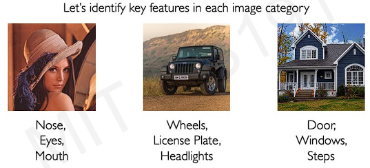
We have to infer that the image is made up of certain classes.
In the image classification, we need to know what patterns we are looking for(1st step), and then we need to detect those patterns(2nd step).
However. difficulties occur when the objects varies.
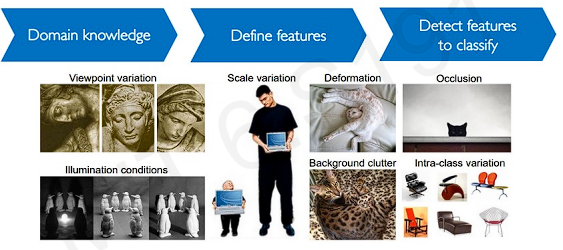
Our model needs ability to handle these various conditions.
Then. how can we make robust algorithm?
Learning Visual features
Before we talk about building algorithm, let's recall fully connected neural network.
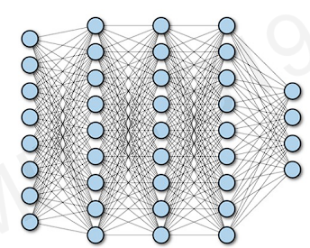
The network has multiple hidden layers, and each neuron is connected to every neuron in its prior layer.
To apply this network into image processing, we firtly have to collapse the image(2D) to a one-dimensional sequence.(known as flatten)
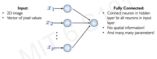
The problem is, spatial information of image is totally lost because we have flattened the image into 1D array. In addition, we have enormous number of parameters because this system is fully connected.
A small image made up of 100 by 100 pixels is going to take 10000 neurons in the first layer.
How can we use spatial structure in the input to inform the architecture of the network?
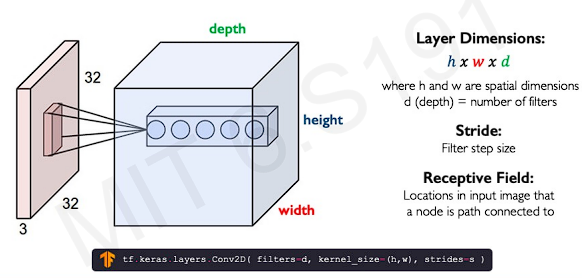
To do this. we first represent 2D image as a 2D array of numbers. Then, we feed the subset of image(the patches) to hidden layer .
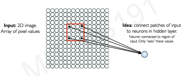
Then we apply this approaches to entire image. We slide the patch pixel by pixel across the input image. We can preserve the spatial information.
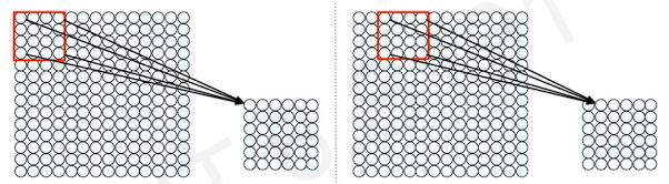
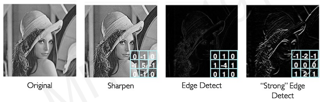
This proccess is called convolution. Here is the example.
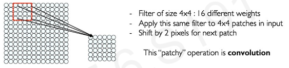
The patch in the picture has 16 different pixels and its weights. Then we use the result of that operation(convolution) to define the state of the neuron in the next layer. After the operation, we move the window(patch or filter) 2pixels for next patch.
Feature Extraction and Convolution
We want to build the convolution algorithm to detect X in the image.
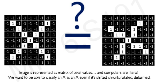
Both of the Xs are X as we can see. But LHS X is rotated to some degree. We want the model to detect both Xs. We need to define the features about X more cleverly. The best way to do is applying convolution.
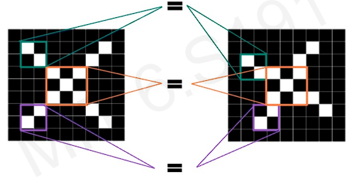
We compare these Xs piece by piece(patch by patch). If our model can detect these rough feature patches in the same position, we can determine these two images are same type or same letter.
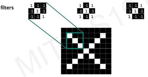
This is the key features to detect X.
Since Convolution method preserves the spatial information, we can detect where important features(The feature can tell Xs whether it is rotated or translated) occur.
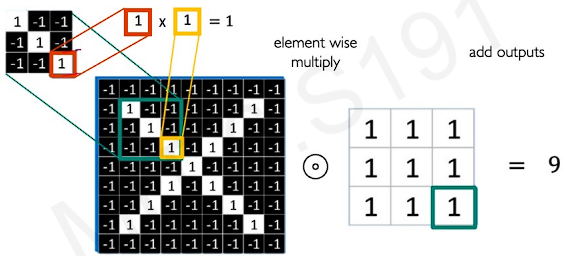
We need to do an element wise multiplication to perform convolution operation.
In short, we have two matrices.
LHS matrix is the weight matrix(the patch) and RHS matrix is the path we are looking to compare it against in our input. And the question is how similar are these two patches.
The outputs of element wise multiplication is to sum up the every location's results.
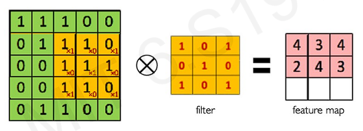
Here is another example.
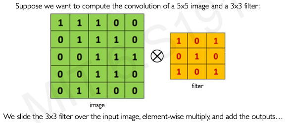
By sliding the filter, we can cover the entire image. We complete the next layer(feature map) by convolutional operation in every slides. And because we use feature map, the spatial information can be preserved.
By changing the weight can achieve drastically different results.
Therefore, we should use multiple filters to extract different features.
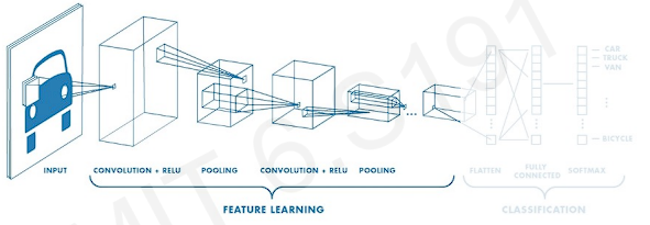
Convolutional Neural Networks(CNNs)
Let's consider a very simple CNN to learn the features for classification.
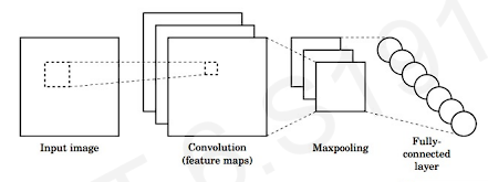
The first step of CNN is the convolution operation to generate these feature maps. These feature maps become inputs.
The second step is applying non-linearity to the feature maps.
And the last step is pooling. The pooling is down sampling operation to allow our images or our networks to deal with larger scale images. We progressivelt down scaling thier size so that our filters can progressivelt grow.
It is difficult story so lets go through more details.
Recall the convolution.
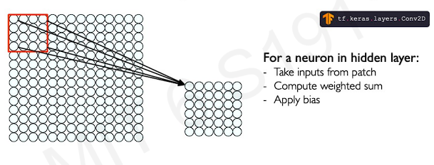
Each neuron in this hidden layer(convolutional layer) is going to be computed as a weighted sum of its inputs applying a bias and activating with a non-linearity(often ReLu). The most important thing in this operation is, every single neuron in this hidden layer only sees a certaion patch of inputs in its previous layer(the image). The next layer, the network will attend to a larger patch and that will not only the red square in the example, but effectively a much larger red square. However, the network will still maintain the ability of detecting in the certain space.
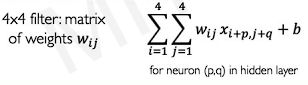
This is the actual equation of convolution operation.
A single convolutional layer is important because it could actually try to detect multiple sets of filters. If anyone wants to detect multiple features in on image, every slices of image effectively denotes a different filter, and each of those filters is corresponding to a specific pattern or feautures.
In these networks, the parameters of node(which is connected to previous image layer) define the spatial arrangement of information and propagates throughout the network and throughout the convolutional layers.
The next step is to take those resulting feature maps and apply a non-linearity. Since the image data is non-linear data, applying non-linearity is really critical.
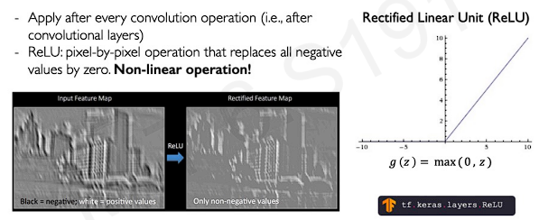
The most common activation function is the ReLU function. As we know about ReLU function, the activation function squashes every neagtive values back up to 0. ReLU is the most common beacause it makes computation easily thanks to its clean derivative.
After applying non-linearity, the next step is pooling. The pooling operation progressively diminishes dimensionality of the image as we go deeper and deeper through convolutional layers.
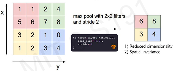
The important thing is as the dimensionality of the image decreases, the dimensionality of filters increases. This is because applying pooling to feature map, the neuron is going to be larger scale of the image.(We call this covering slices as receptive field. We can easily understand this notion by the figure)
A very common technique for pooling is what's called maximum pooling(or Max pooling). Instead doing convolution operation, what this pooling do is simply take the maximum of the patch location. It makes neural network to propagate only the maximums. There are many other ways for downsampling(mean pooling / average pooling)
Here is the example of CNNs working.
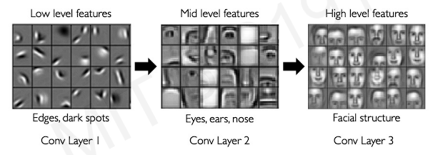
We can see receptive field grows as the dimensionality of filters grow through the convolutional layers. These process is also called as hierarchical decompositions.
In conclusion the following figure shows two step of image processing(learning features, and detecting features).
First step
- Learn featurs in input image through convolution
- Introduce non-linearity through activation function(real-world data is non-linear!)
- Reduce dimensionality and preserve spatial invariance with pooling
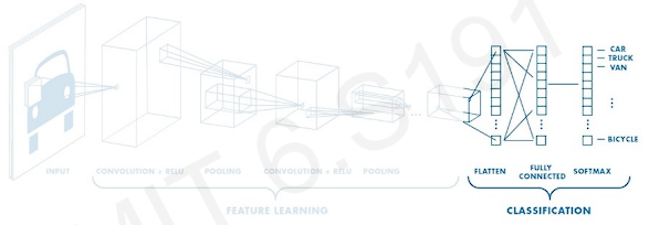
Second step
- CONV POOL layers output high-level features of input
- Fully connected layer uses these features for classifying input image
- Express output as porbability of image belonging to a particular class
- softmax function :
->softmax function maintain the output properties between 0 to 1 and positive.
This is the code for simple CNNs
import tensorflow as tf

def generate_model():
  model = tf.keras.Sequential([
  	# first convolutional layer
  	tf.keras.layers.Conv2D(32, filter_size=3, activation='relu'),
  	tf.keras.layers.MaxPool2D(pool_size=2, strides=2),

  	# second convolutional layer
  	tf.keras.layers.Conv2D(64, filter_size=3, activation='relu'),
  	tf.keras.layers.MaxPool2D(pool_size=2, strides=2),

  	# fully connected classifier
  	tf.keras.layers.Flatten(),
  	tf.keras.layers.Dense(1024, activation='relu'),
  	tf.keras.layers.Dense(10, activation='softmax'), # 10 outputs
  ])
  return model
At second layer, we keep progressively exapand the set of pattern, and finally flatten those resulting features.
An Architecture for Many Applications
This architectures(simple CNNs) are extensible and they extend to so many different applications and model types. Especially we can utilize the first part of CNNs into any other task like object detection, segmentation, probabilistic control.
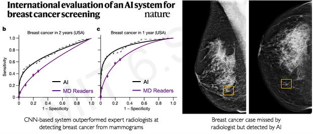
example 1. classification : Breast cancer screening
example 2. object detection
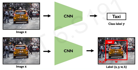
The neural network can not only identify what it is but also find bounding box of the target. The task is both a regression problem(where is the box -> continuous problem) and classification(what is in that box)
The model can be extended for much harder problem such as multiple detection.
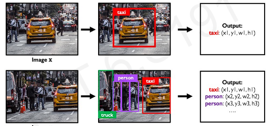
However, in real-world image, it has so many different possibilities of object(different size of box, different objects).
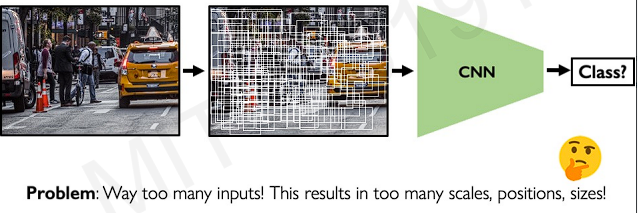
To solve the problem, we take the box where it is high likelihood of having an object might be presented. Then we feed in those high attention locations to our convolutional neural network. But this algorithm still has problems.
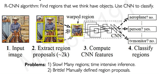
There is improved version of R-CNN(faster R-CNN). A image feed into region proposal neworks. The goal of the networks is to propose certain regions in the image that we should attend to then feed just those regions. In other words, the goal is to learn or extract all of those key regions and process them through later part of the model.
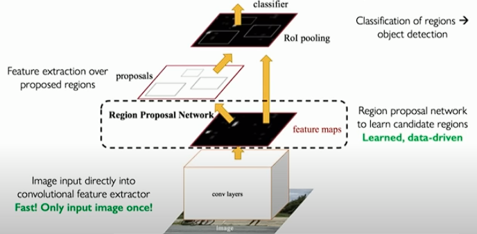
The faster R-CNN is fast enough to use in the real-world.
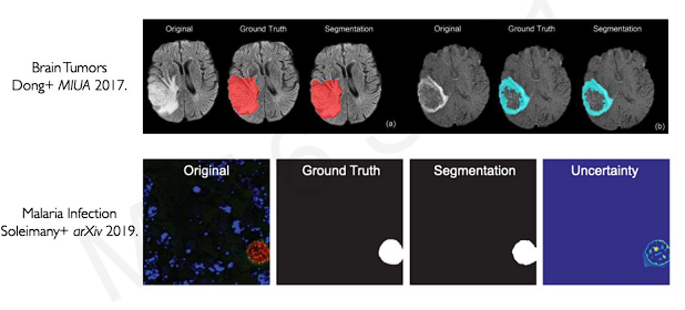
example 3. semantic segmentation : Fully Convolutional Networks
In this task, we classify every single pixel in the image.
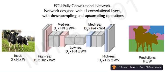
The example shows where the pixel belongs to(cow, trees, grass, or sky) and the goal of the model is to reconstruct the space into a new space of semantic labels.
This can be applied to healthcare problem.