Why Deep Learning?

machine learning : human have to define features

-> it is time consuming, brittle, and not scalable in practice

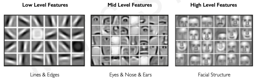
deep learning can extract and uncover what are the core patterns in the data directly

• for example, deep learning can extract low level features, and then combine into higher level.

Why Now?

1. datas become more pervasive. More data is available(Big Data)

2. Deep Learning requires a lot of compute. According to hardware advances, large training algorithm became possible.

3. By open source software(tensorflow), we can easily train and build the code for Deep Learning neural Network

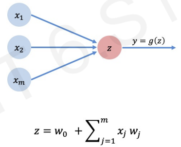
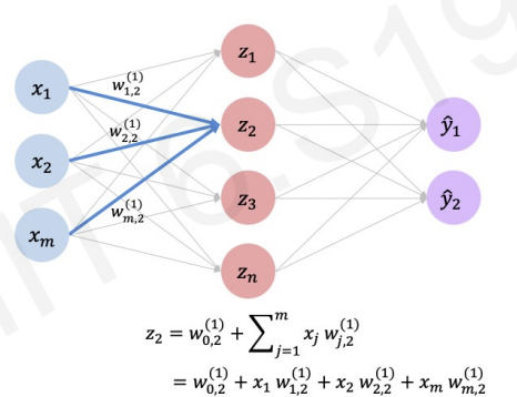
The perceptron : The structural building block of deep learning

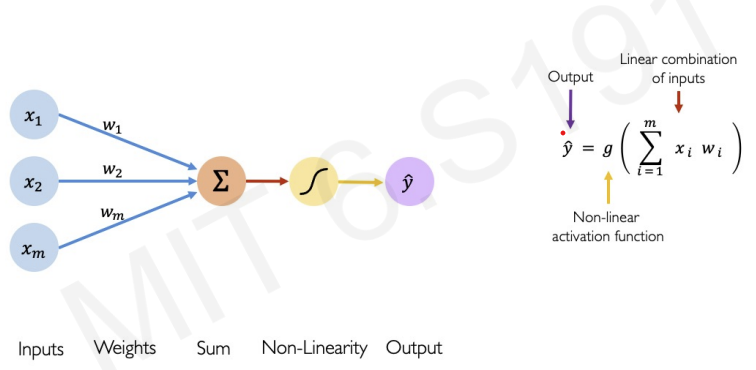
left(blue circles) : M different inputs -> multiplied by a corresponding weight ($x_1 w_1$)
-> add all of its inputs -> pass through non-linear activation function -> output $\hat{y}$ : perceptron

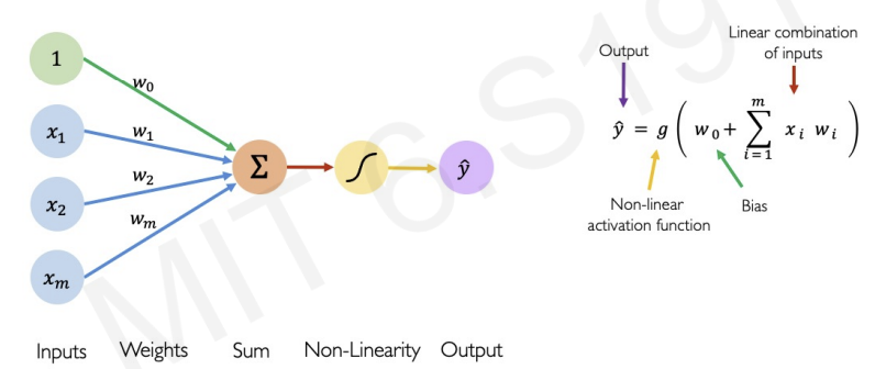
for more accurate definition we add bias

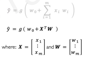
by applying linear algebra, we can rewrite the equation.(Matrix Multiplication)

What is Activation Functions?

Activation Functions in deep learning are mathematical equations that determine the output of a neural network.

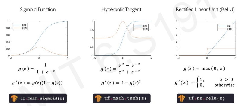
sigmoid : can deal probability distribution between 0 and 1
ReLu : efficient to compute especially when its derivatives are constants

Why do we need activation functions?

to introduce non-linearities to our data(almost all data in real world is highly non-linear)

-> so we need nonlinear model to capture patterns

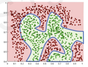
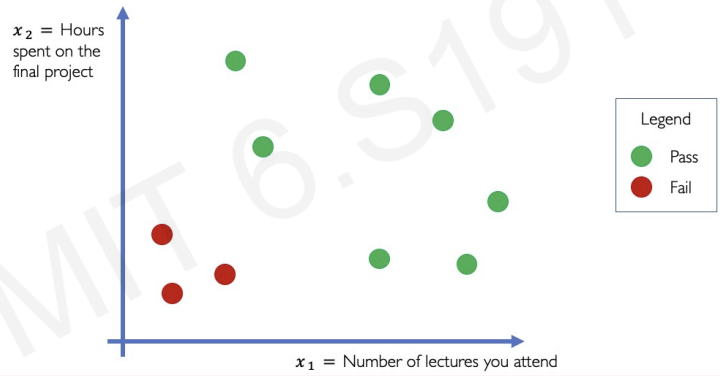
example problem : we want to separate red points & green points

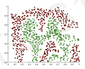
if we apply linear function, it is not satisfying.

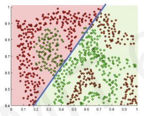
This is why we need non-linearity (activation functions)

example of the perceptron

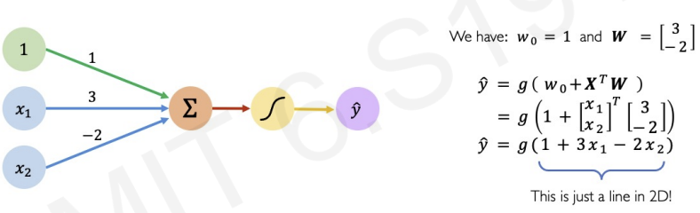
as mentioned earlier, we need 3 steps.
1. multiply inputs and their corresponding weight.
2. add thier results.
3. compute a non-linearity

we call it forward propagation

In this case, we can plot the result(2 dimensional line).

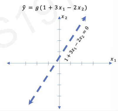
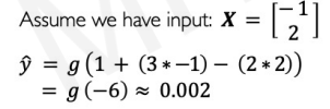
If the activation function is sigmoid, then we get z < 0.
By visualized plot, we can understand activation function separating two areas.

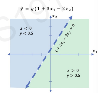
however, most datas are not feasible to visualize

Building Neural Networks with Perceptrons

before we build neural networks, let's simplify previous concept

we define z as sum of inputs(multiplied by its weight) and add bias($w_0$)

now, with this concept, we can build multi-layered output neural network(by stacking the perceptrons!)

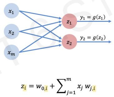
in this picture, all inputs are densely connected to all ouputs. We call this Dense layers.
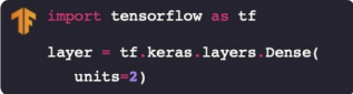
the code from this mathematical understanding :

class MyDenseLayer(tf.keras.layers.Layer):
	def __init__(self, input_dim, output_dim):
    	super(MyDenseLayer, self).__init__()
        
        #Initialize weights and bias
        self.W = self.add_weight([input_dim, output_dim])
        self.b = self.add_weight([1, output_dim])
        
    def call(self, inputs):
    	#Forward propagate the inputs
        z = tf.matmul(inputs, self.W) + self.b
        
        #Feed through a non-linear activation
        output = tf.math.sigmoid(z)
        
        return output

we can use library to build neural networks without implementing

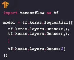
• We can also make more complex neural networks
  

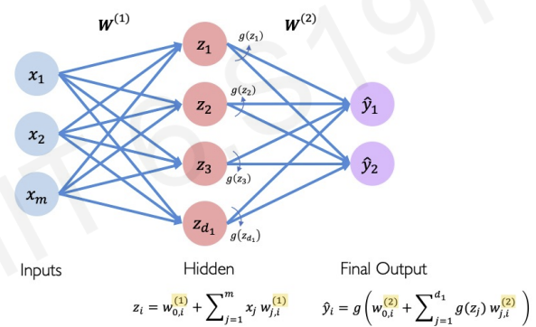
In the hidden layer, each z are determined by each weight matrix and bias. For example, $z_2$ has its unique weight matrix and bias.

we can simplify this concept by this figure :

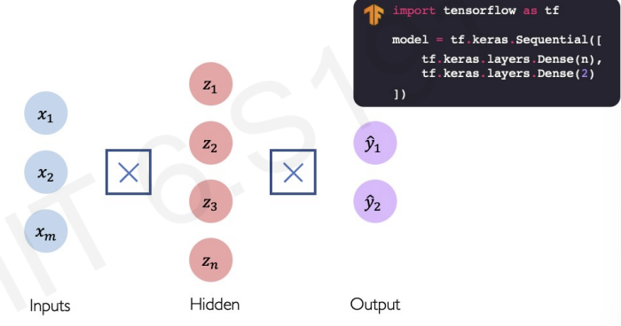
• by Sequential model library, we can add additional Dense layer(The new layer is output from prior layer. Not from neuron layer!).

• we can make deep neaural network by stacking these Dense(hidden) layer.
  
  

Applying Neural Networks

example problem - 2 inputs

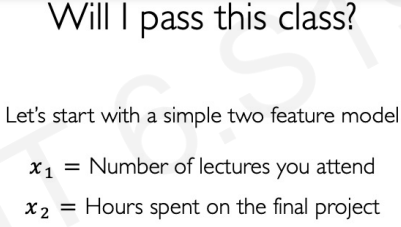
after collecting data, we plot the data

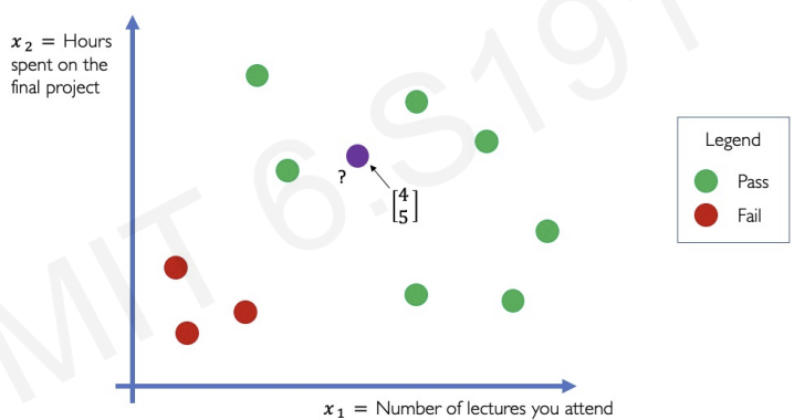
If we met unseen data(purple point) we need prediction from neural network.

we build the neural network as single-layered neural network

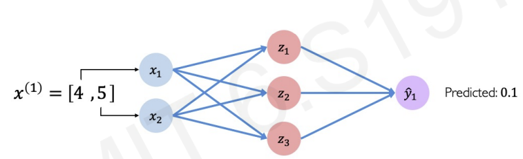
The prediction result is 0.1 but actual result is 1.
Why this difference occured?

this neural network is not trained about the world, this class. So it has no information about meaning of pass or fail. It just calculate multilpication and addition

we should tell neural network the answer, if it makes a mistake.

neural network will make better prediction to minimize the mistake.
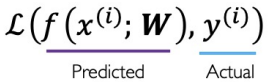
In neural network, the mistake is called losses.
We need to define loss function that tells how big of a loss there is.

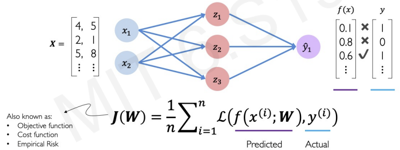
In deep learning, loss function is also called cost function, objective function, empirical risk.

For instance, in binary classification(Yes or No problem), we define cost function like this :

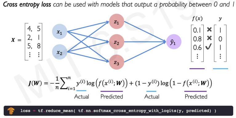
we can calculate the loss by cross entropy.
What is cross entropy and softmax?
softmax : The softmax function is commonly used for multi-class classification problems. The inputs are normalized into probabilities.

cross-entropy : Cross-entropy is a measure of the difference between 2 probability distributions.

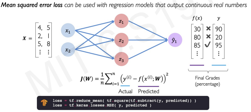
Another loss function is mean squared error loss that can be used with regression models that output continuous real numbers.

Training Neural Networks

we want to find the network weights($W$) that achieve the lowest loss.

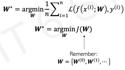
$W^{*}$ is the list of networks weights that minimize average of losses

for example, let $J(W)$ as loss function of two weight neural network that can be visualized in fugure.

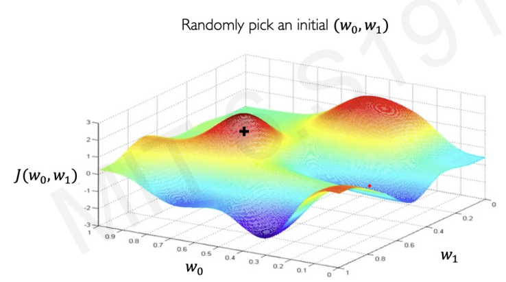
Then, let's find the set of $W$ that minimize $J(W)$.
First, we pick random point $(w_0, w_1)$ and compute gradient at that point.(The loss function is continuous, so we can compute gradient)

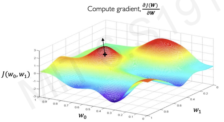
The direction of gradient tells us where we should go to increase our loss.
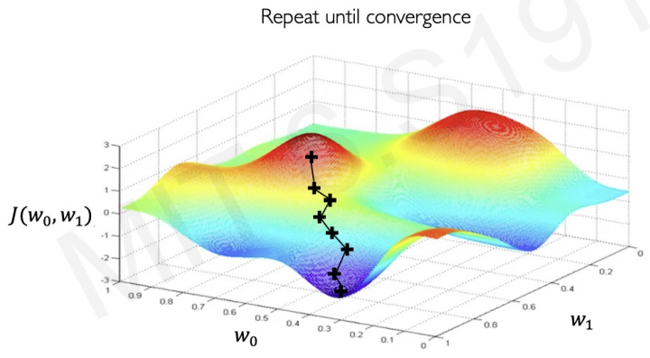
Therfore, we take small step in opposite direction of gradient.
Repeat this step until we met minimum point(convergence)

recall gradient descent algorithm

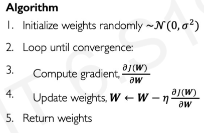
after computing gradient, we need to choose step size for updating weights. This step size is also called as learning rate.

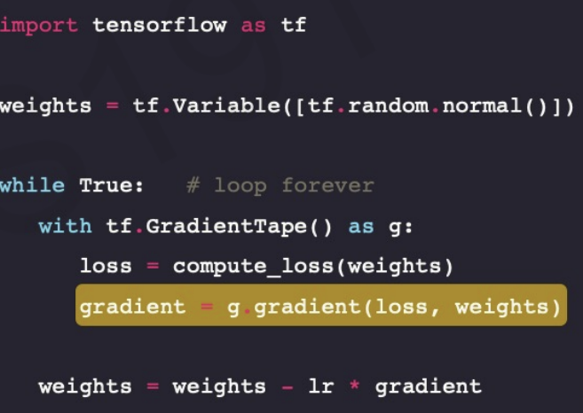
we can calculate gradient easily by the library.
The underlined code is the process of updating weights, this is called back propagation.

We can understand backpropagation with simplest neural network.

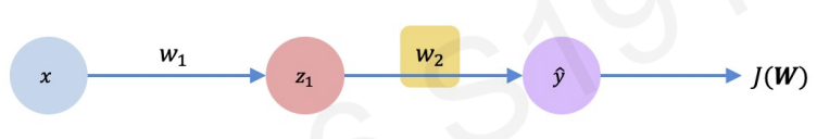
The figure has one input, one neuron, and one output.
If we change one weight(for example : $w_2$), how does it affect the final loss $J(W)$?

Before we change the weight, we need partial derivative of $J(w)$.(Let's apply chain rule!)

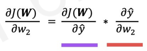
we can also apply this chain rule to get partial derivative with respect to $w_1$.

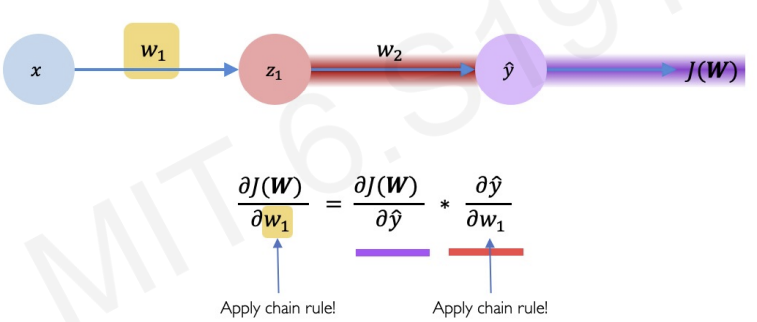
then, we finally get full partial derivative by expanding chain rule.

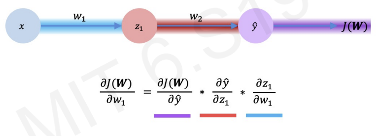
We first compute the partial derivative with respect to $w_2$, and then we back propagate and use that information also with $w_1$.
This process is called back propagation.(occurs from the output all the way back to the input)
To be specific, we update the weight $w_1 = w_1 - \alpha \frac {\partial J(W)}{\partial w_1}$.($\alpha$ is learning rate)
To determine for every single weight, we need to repeat this process for every weight in the network using gradients from later layers.

Neural Networks in Practice: Optimization

Most of deep neural network is difficult to train(optimize)

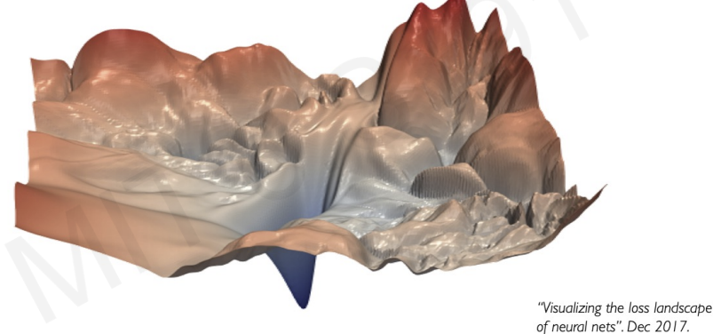
This figure tells a landscape of one of the neural network.
It seems hard to find minimum point.

Recall weight update equation.

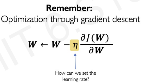
A constant corresponding to gradient is called Ada, known as learning rate.
Setting this value of learning rate is very challenging.

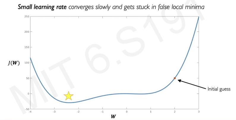
1. If the learning rate is too small, it not only converges slowly, and even do not converge to global minimum.
   -> can be stuck at global minimum.
2. If the learning rate is too big, it starts to diverge from the solution.
   -> can explode!
3. We need appropriate medium value

How to deal with this?

Idea 1. Try lots of different learning rates and see what works "just right".
Idea 2. Design an adaptive learning rate that "adapts" to the landscape.

To be specific in Idea 2, we need to consider
$1$ how large gradient is
$2$ how fast learning is happening
$3$ size of particular weights
$4$ etc..

There are many algorithm(SGD, Adam, Adadelta, Adagrad), many TF Implementation for determining the value of learning rate.

Here is the code that covers everything we learned today.

import tensorflow as tf

model = tf.keras.Sequential([...])

'''pick your optimizer(with regard to conditions such as how large gradient is, how fast learning is happening,...)'''
optimizer = tf.keras.optimizer.SGD()

while True: # loop forever
	
    #forward pass through the network
    prediction = modle(x)
    
    with tf.GradientTape() as tape:
    	#compute the loss
        loss = compute_loss(y, prediction)
        
    #update the weights using the gradient
    grads = tape.gradient(loss, model.trainable_variables)
    optimizer.apply_gradients(zip(grads, 
    model.trainable_variables))

Neural Networks in Practice: Mini-batches

In real world, computing $\frac {\partial J(W)} {W}$ is very computationally intensive.
$\because$ it is computed as a summation across all of the pieces in our data set(data set is too large!).

Instead of computing gradient across the entire data set, we can compute the gradient over just a single example in our data set.

It computes much faster, but it can be noisy and roughly reflect trend of the entire data set. This is called stochastic gradient descent(noisy).

We can apply middle ground idea. Instead of computing it with respect to just one example, we can compute the gradients over some small example, called mini batches.

Since the mini batch is not large, it is still computationally efficient. The stochasity will be reduced, and the accuracy of our gradient will be much improved.

Another advantage of mini-batches is that we can parallelize computation by splitting the set of mini batches.
-> We can achieve significant speed increases on GPU

Neural Networks in Practice: Overfitting

We want to design a model that can accurately describes some patterns in data never seen before(test data).

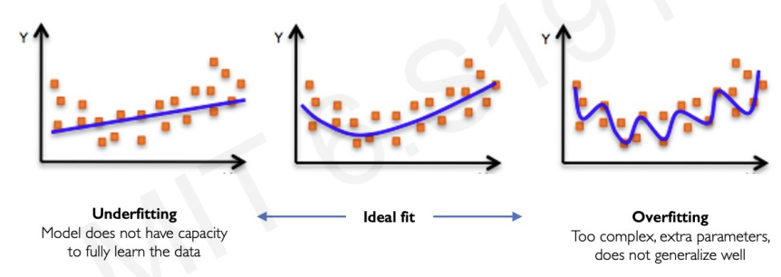
If the neural network is simple, like one straight line,the model cannot explain the patterns of data.
On the other hand, if neural network is much complex, it is not actually not representative of test data.

we need middle ground.

How to achieve the middle ground?
-> By applying regularization.
It is technique that constrains our optimization problem to discourage complex models.

1. The most popular method of regularization : Dropout

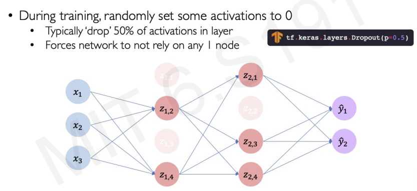
In this figure, we control how many layers activate in training. We set 50% of layers to activate. At each iterations(outer loop), we randomly turn them off. Therfore, every iteration provides different model that not only learn how to build internal pathways to process the same information, but also not rely on information that it learned on previous iterations.
we can think of this regularization as ensemble of different models from iterations.
Dropout reduce the model's capacity(which means it prevents overfitting), and train much faster because of its less layers.

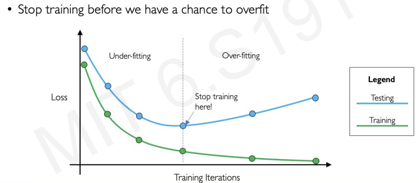
2. Second method of regularization : Early stopping