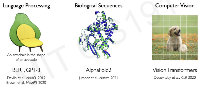
Deep Sequence Modeling

In this page, we are focused on specific types of problems that involves sequential processing of data

What is the sequential data?

If we want to predict a direction of a ball without any information(it's history, the trajectory of the ball, it's motion), the prediction is going to be a random guess.

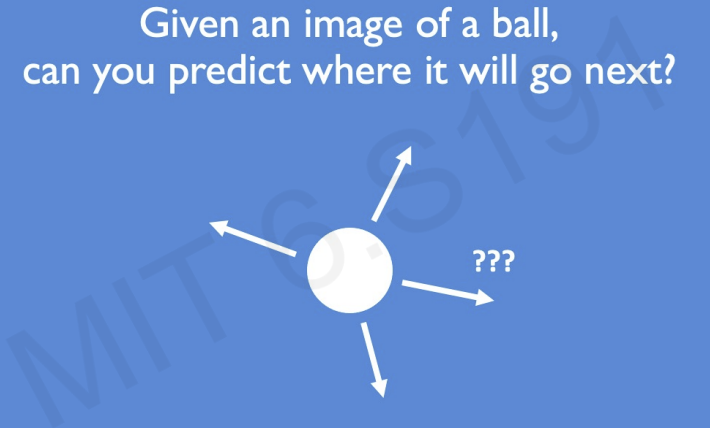
However, if we are provided additional information(where it was moving in the past), the problem becomes musch easier.

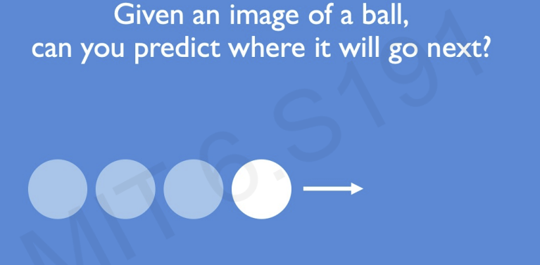
This data is called sequential data
Another example of sequential data is audio data.

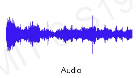
The sounds form a sequence of sound waves. We can split up to think about in this sequential manner.

Text language can also be split up into a sequence of characters or a sequence of words.

There are so many other examples of sequential data.
financial markets, medical signals, etc..

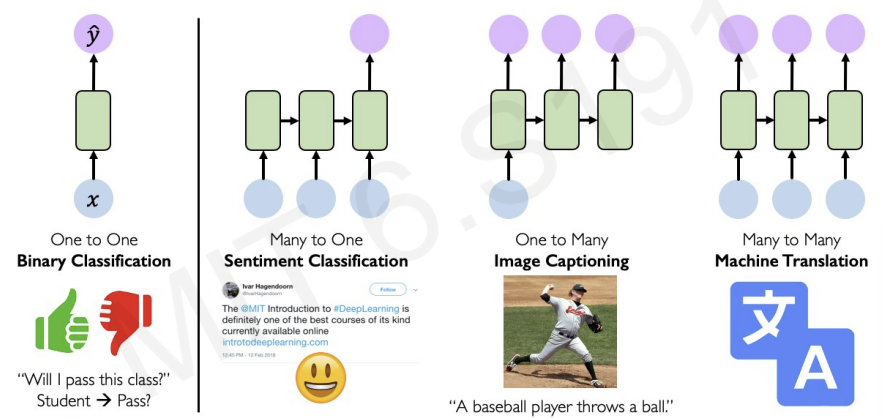
The classification model has one to one structure.
-> one input provides one output.

In the sequece models, they have various structure.

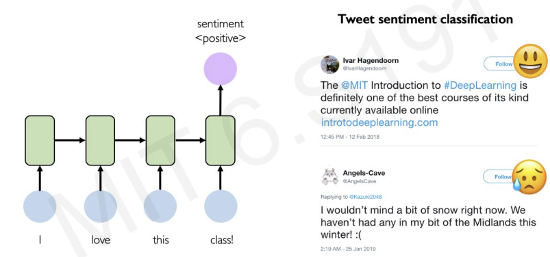
• text language inputs(many) -> whether it is good sentiment or bad sentiment(one).
• Image input(one) -> describe the picture in text language(many).
• translate between 2 languages(many to many).

Neurons with Recurrence

recall the neural network with stacking the perceptrons.

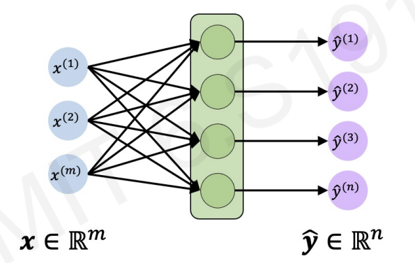
Even though we can make multiple outputs by applying weight operations and non-linearity, we cannot still achieve time processing data, or sequential information.

Before we go through next step, let's simplify the figure.

The green area is the single layer shown in the previous figure.

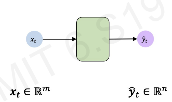
How can we make this model as time processing model?

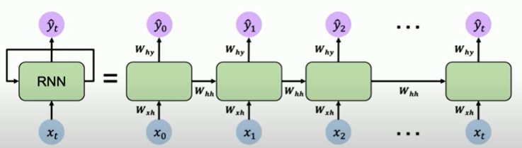
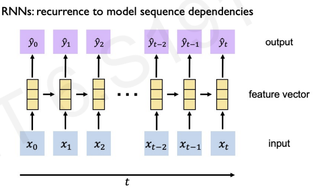
we can repeat the process by feeding in different input vector corresponding to different times.
As we have individual time step starting with $t_0$, we first fed in $x_0$ and do the same operation for the next time step.

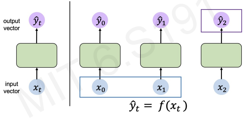
The equation tells us the predicted output($\hat{y}_t$) at a particular time step
The later predicted output($\hat{y}_2$) could depend on previous inputs($x_0, x_1$)

Then, how could we define a relation that links the Network's computations at a particular time step to prior history?

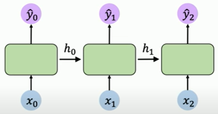
we link the computation & information to other replicas(same neural network) via recurrence relation

The recurrence relation is the computation at a particular time is passed on to those later time steps, denoted as $H$

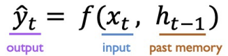
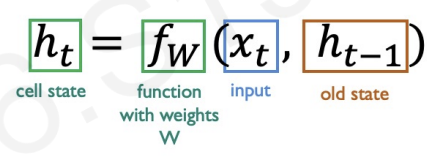
conclusion : as we need to consider another variable $H$, the equation becomes $\hat{y}_t = f(x_t, h_{t-1})$
The variable H is array of parameters : $h_t$

we can also simplify the previous figure.

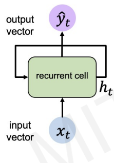
$h_t$ updates after making prediction $y_t$, and then fed into the same neural network. (we can think as recurrence relation)
This recurrence relation is called recurrent neural networks(RNN).

Recurrent Neural Networks(RNNs)

RNNs have a state, $h_t$, that is updated at each time step as a sequence is processed

how can we update $h_t$?

-> the same function and set of parameters are used at every time step($f_W$)

RNNs in python

my_rnn = RNN()
hidden_state = [0,0,0,0] #Initializing 

sentence = ["I", "love", "recurrent", "neural"]

for word in sentence:
	prediction, hidden_state = my_rnn(word, hidden_state)
    
next_word_prediction = prediction

every for loop : prediction = $y_t$, hidden state = $h_t$
next_word_prediction = final output

equations for RNNs

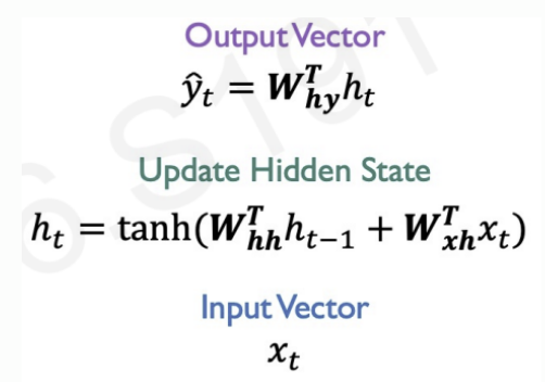
In updating equation : previous hidden state is multiplied by a weight matrix, and input vector is multiplied by another weight matrix, and they pass through non-linearity.

$W_{hh}$ is a weight matrix for transforming $h_{t-1}$ into $h_t$
$W_{xh}$ is a weight matrix for transforming $x_t$ into $h_t$
$W_{hy}$ is a weight matrix for transforming $h_t$ into $y_t$
We reuse the same weight matrices at every time step!

$tanh$ is a one example for non-linearity.(it can be other functions like ReLu)

The figure tells more details.(about weight matrices)

How we define the loss?

We define $L_t$ as a loss that is computed from a prediction at an individual time step.(loss between $y_t$ and $target_t$)

Then, we can get our total loss by taking all these individual loss terms and summing them.

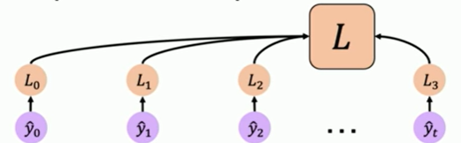
after computing total loss, we update weight matrix by backpropagation to minimize the loss.

RNNs implementation in TensorFlow

class MyRNNCell(tf.keras.layers.Layer):
	def __init__(self, rnn_units, input_dim, output_dim):
    	super(MyRNNCell,self).__init__()
        
        #Initialize weight matrices
        self.W_xh = self.add_weight([rnn_units, input_dim])
        self.W_hh = self.add_weight([rnn_units, rnn_units])
        self.W_hy = self.add_weight([output_dim, rnn_units])
        
        #Initialize hiddent state to zeros
        self.h = tf.zeros([rnn_units, 1])
        
    def call(self, x):
    	#Update the hidden state
        self.h = tf.math.tanh(self.W_hh = self.h + self.W_xh * x)
        
        #compute the output
        output = self.W_hy = self.h
        
        #Return the current output and hidden state
        return output, self.h

in the call function, the parameter x is the input vector. We first update hidden state from the equation, then compute the output, and return these updated output and hidden state.

Another way to make RNN is using implemented library.

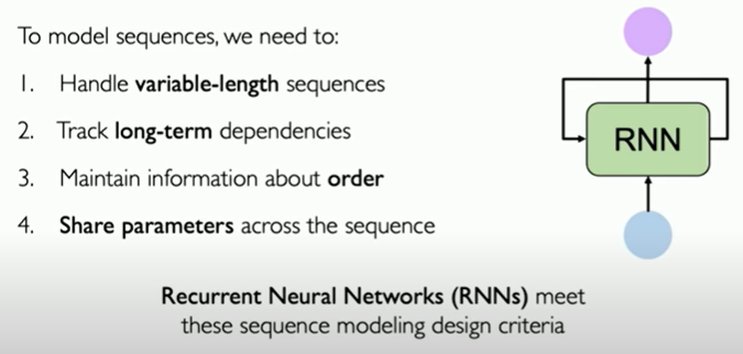
tf.kera.layers.SimpleRNN(rnn_units)

To model sequences, we meet modeling design criteria
1. Handle variable-length sequences
2. Track long-terms dependencies
3. Maintain information about order
4. Share parameters across the sequence

Following examples will show more specific details about these design criteria.

A Sequence Modeling Problem : Predict the Next Word

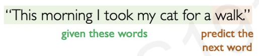The task is predicting the last word in the sentence.

The first step to design the model is representing language to a Neural Network. This is because, computer cannot interpret words.

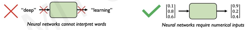
To represent the words into numbers, the key solution is embedding. Embedding transforms indexes into a vector of fixed size.

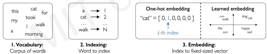
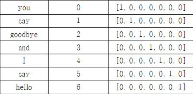
First, we define all the possible words that could occur in this vocabulary. Then we map these individual words to a numerical vector(fixed size). The mapping is also called one-hot-embedding.
another example :

After embedding done, we need to handle sequence length (The sequences can be long or short) and track dependecies across all these different lenghts.

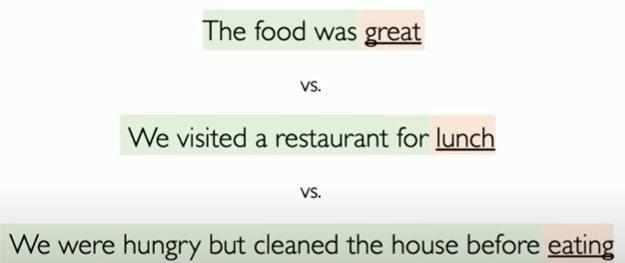
Dependencies are important beacause the same words in a compeletly different order have completely different meanings.

To sum it up, we need to follow four steps.

To follow these steps, we need information about BPTT

Backpropagation Through Time(BPTT)

In RNNs sequence, we need to backpropagate the loss through each of these individual time steps.($\because$ the loss of RNNs is the sum of loss at individual time steps)

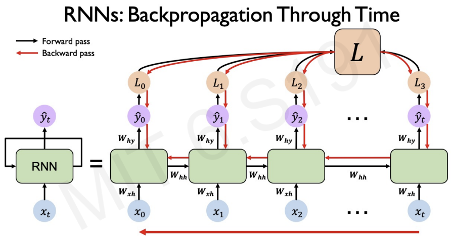
After back propagating loss through each of the individual time steps, we then back propagte across all time steps(from current time $T$ to beginning of the sequence, updating $W_{hh}$).
However, backpropagating through time steps is quite tricky.

As I learned, backpropagation needs chain rule.
Computing the gradient with respect to $h_0$ involves many factors of $W_{hh}$ and have to repeat computation.
The problem is, if the weight matrix $W$ is very very big, the gradients will be explode or vanish easily.

• If many values in weight matrix are bigger than 1, the gradients explode.
• If many values in weight matrix are smaller than 1, the gradients vanish.

Simple solution for exploding gradient is clipping gradients to constrain them.
Gradients vanishing is a very real problem.
Why?

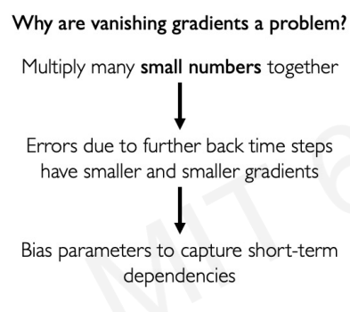
If the sequence gets longer, vanishing gradients make RNNs unable to establish long term dependencies.
To handle gradients vanishing, we have several tools.
1. Activation function
2. Weight initialization
3. Network architecture

Trick #1 : Activation Functions

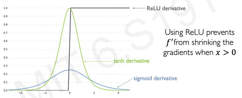
Recall ReLu function's shape. In contrast to sigmoid or tanh, ReLu derivative is 1 in all instances where $x$ is greater than 0. This alleviates gradient vanishing problem.

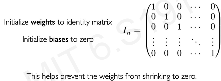
Trick #2 : Parameter Initialization

Trick #3 : Gated Cells(The most robust solution)

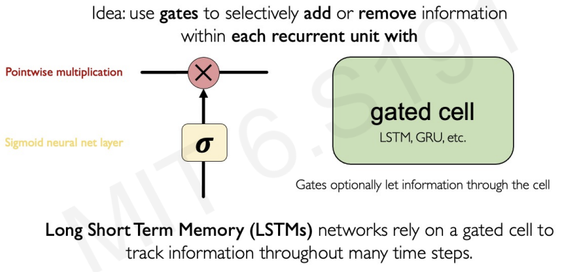
The gate controls selectivley the flow of information into the neural unit. -> This makes neural units filter out what is not important while maintaining what is important.

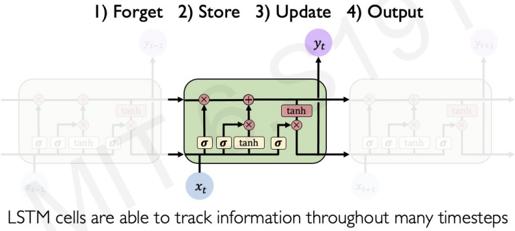
Key Concepts of LSTMs:
1. Maintain a cell state
2. Use gates to control the flow of information

• Forget gate gets rid of irrelevant information
• Store relevant information from current input
• Selectively update cell state
• Output gate returns a filtered verstion of the cell state

3. Backpropagation through time with partially uninterrupted gradient flow

We can call LSTM in python by a code :

tf.keras.layers.LSTM(num_units)

RNN Applications & Limitations

Example Task : Music Generation

Input : shett music -> Output : next character in sheet music

Example Task : Sentiment Classification

Limitations of RNNs(including LSTMS):
1.Encoding bottleneck
-If input text has many different words and the output is just single value, encoding may be very very challenging and lots of information can be lost!
2.Slow, no parralelization
-There is no easy way to parrelize computation.
3.Not long memory
-The capacity for maintain long-term memory is actually not that long.

Desired capabilities : we want continuous stream / parallelization / long memory

How can we beyond these all time step?

A naive approach would be to squash all the data & all time steps together.(concatenating feature vectors)

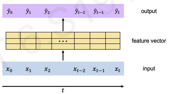
Even though we eliminated recurrence, other limitations still exists.(Not scalable / No order / No long memory)

More clever approach : identify and attend to what is important! (attention notion)

Attention

attention is the foundational mechanism of the Transformer architecture

let's see image example

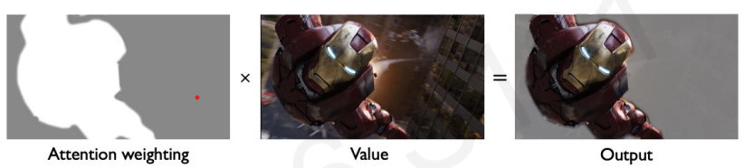
our goal is to extract the most important parts of an image.
We(human) can just see the iron man and then extracting the important features.

The goal for attention is to act like we do
1.Identify which parts to attend to(similar to a search problem!)
2.Extract the features with high attention

Then, how do we search?(identifying)
Following example will show the details.

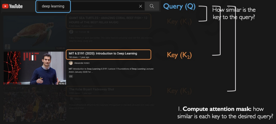
aftet we enter the query(inputs), the algorithms find the overlaps between entered query and each of these titles. It computes metric of similarity and relevance between the query and keys.

let's see the process by another example.
Here is a task for identifying text sequence.

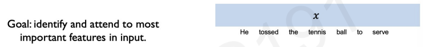
First, we do encoding position information(eliminating recurrence by adding position information) -> can process time steps all at once!

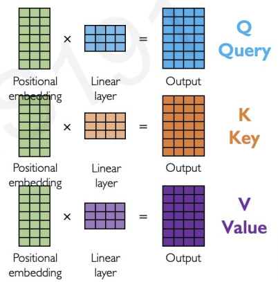
Second, we extract query, key, value for search(just like upper example : iron man)
we do this by separating neural networks for query, key, value with different weight matrices.

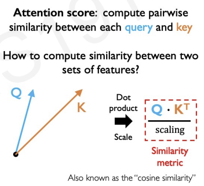
Third, compute a similarity score between the query and the key. The query and the key are already encoded into vectors.
We can compute similarity by the dot product and scaling.(whether or not they are pointing in the same direction)
These metric is also called cosine similarity.(In linear algebra)

The vectors can also be represented as matrices.

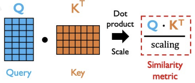
In our example, we compute similarity score metric

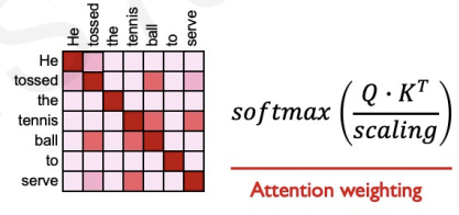
The softmax function constrains those similarity values to be between 0 and 1.

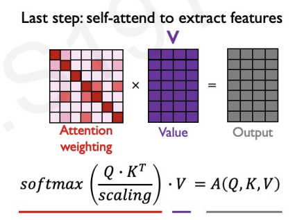
Finally, we multiply value matrix to get extracted feature(output).

We can apply this procees into iron man example.

self-attention is applied to many different models.