각 연산들을 수행하는데 걸리는 평균 수행 시간을 나타낸다.
Amortized analysis 를 사용하는 이유는 T(n)=O(n) 인 경우, 항상 O(n)의 연산이 발생하는 것이 아니라 대부분 O(1)의 연산으로 처리되는데 모든 연산을 O(n)으로 처리하는 것이 아깝기 때문이다.
여러 연산 중 특정 연산의 시간복잡도가 매우 커도 개별 연산자들의 시간복잡도를 평균적으로 보면 효율적이게 동작함을 보일 수 있다.
Worst case에도 개별 연산자에 대한 평균적인 비용은 효율적임을 보일 수 있다.
Amortized Analysis 의 방법
1. Aggregate analysis
n개의 임의의 시퀀스가 있을 때, : i번째 연산을 수행하는 데 걸리는 실제 수행 시간이라고 하자
를 만족하는 T(n), 즉 upper bound 를 찾아 T(n)/n 을 구하는 방법
이 방법에서는 모든 각각 연산의 평균적인 수행 시간은 동일하다.
Example of Aggregate analysis
1. Stack operation
- push: O(1)
- pop: O(1)
- multipop: O(n), stack이 가득 차 있는 경우
MULTIPOP(S, k)
	while not STACK-EMPTY(S) and k>0
    	POP(S)
        k = k - 1

// cose of MULTIPOP(S, k) 는 O(k) 이다.
// 만약 k가 현재 stack 에 들어있는 데이터 개수보다 크다면
// O(현재 stack 에 들어있는 데이터 개수)
T(n) 을 구하자
- n개의 연산은 PUSH, POP, MULTIPOP 으로만 이루어져 있다.
- MULTIPOP은 k개의 POP과 다를 바 없다.
- #(push) #(pop)
- #(push) #(pop)
- T(n) = O() = O(n)
Amortized cost
=
이를 통해 stack operation(PUSH, POP, MULTIPOP)의 worst case: O(n) (multipop(S, n)) 이지만, amortized analysis를 통해 평균적으로는 O(1)임을 확인할 수 있다.
2. Incrementing binary bit counter
A[0]이 가장 낮은 자리를 나타내는 A[0...k-1] 을 k-bit binary counter로 생각하자.
INCREMENT(A) //0...2^k-1
	i = 0
    while i < A.length and A[i] == 1
    	A[i] = 0 //Bit flip, O(1)
        i = i + 1
    if i < A.length
    	A[i] = 1 //Bit flip, O(1)
각 INCREMENT operation의 cost는 직전 binary code와 비교해서 bit flip 된 bit의 개수이다.
T(n) 을 구하자
- 각 INCREMENT operation의 시간 복잡도는 최대 k개의 bit flip이 발생할 수 있기 때문에 O(k)이다.
- INCREMENT operation의 개수는 이다.
- 전체의 upper bound는 이다.
위 T(n)보다 tight한 upper bound를 구할 수 있다.
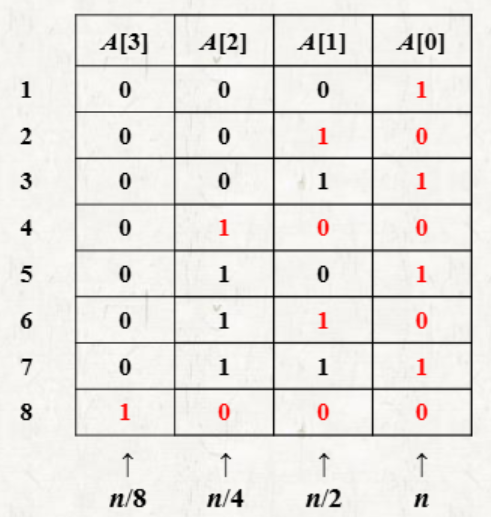
- 그림을 보면 A[0] = n번, A[1] = 번, A[2] = 번 bit flip이 발생한다.
- 이를 일반화하면 A[i] = 번 bit flip이 발생한다.
- Tighter upper bound
Amortized cost
이를 통해 INCREMENT 연산의 worst case: O(k) (All bits are flipped) 이지만, amortized analysis 를 통해 평균적으로는 O(1)임을 확인할 수 있다.
2. Accounting method
Aggregate analysis와 다르게 여러 개의 연산 유형이 존재할 때, 각 유형에 맞게 amortized cost를 부여하는 방법
각 연산의 amortized cost가 actual cost 보다 크면 된다.
: amortized cost, : actual cost 일 때,
을 만족해야한다.
위와 같은 부등식을 만족해야하는 이유는 특정 연산에서 amortized cost - actual cost 가 음수라면 다른 연산에서 남는 cost(credit)를 사용할 수 있도록 하여 total cost가 유지될 수 있도록 하기 위해서이다.
Credit = -
Total credit =
각 연산 진행 후 credit도 자료구조에 같이 저장한다.
Example of Accounting analysis
1. Stack operation
-
Actual cost
- PUSH: 1
- POP: 1
- MULTIPOP(S, k): min(k,s)
-
Amortized cost
- PUSH: 2
- POP, MULTIPOP = 0
-
PUSH credit = 2 - 1 = 1, 이 credit은 POP, MULTIPOP에 사용된다.
- POP, MULTIPOP은 항상 PUSH 이후에 실행되므로 가능하다.
-
Credit은 음수가 될 수 없다.
- stack은 nonnegative objects 이기 때문이다.
- 따라서 the total amortized cost 는 total actual cost의 upper bound 이다.
Total amortized cost: O(2n) = O(n)
Total actual cost: O(n+m) = O(n)
2. Incrementing binary bit counter
- Actual cost
- Bit set(0->1): 1
- Bit reset(1->0): 1
- Amortized cost
- Bit set(0->1): 2
- Bit reset(1->0): 0
- Bit set credit = 2 - 1 = 1, 이 credit은 Bit reset에 사용된다.
- Bit reset은 항상 Bit set 이후에 수행되기 때문에 가능하다.
- Credit은 음수가 될 수 없다.
- Counter의 1의 개수는 nonnegative 이기 때문이다.
- 따라서 the total amortized cost 는 total actual cost의 upper bound 이다.
Total amortized cost: O(n)
Total actual cost: O(n)
Running time: O(n)
3. Potential method
Accounting method와 비슷하지만 credit 대신, potential 을 사용한다는 점에서 차이가 있다.
Credit: 각 연산마다 데이터 구조 내의 특정 객체나 연산에 할당된다.
- each credit is associated with a specific object within the data structure
Potential: 특정 객체나 연산에 대해 설정된 것이 아니라, 데이터 구조 전체의 "상태"를 나타낸다.
- The potential is associated with the whole data structure
Credit은 각 연산마다 자료구조에 같이 저장된다면, Potential은 전역 변수로써 존재한다고 생각할 수 있다.
: Initial data structure
: i번째 operation을 적용한 후의 data structure
: 에 해당하는 potential
Potential difference
i번째 operation을 수행하고 Potential의 차이
- 양수
- The potential of the data structure increases
- 음수
- The decrease in the potential pays for the actual cost of the operation
Amortized cost
Total amortized cost
=
=
Accounting method에서와 같이 ( 이 성립해야 한다.
- 이 모든 i에 대해 성립해야 한다.
Example of Potential method
1. stack operation
- 는 i번째 operation 이후 stack에 들어있는 데이터의 개수이다.
- = 0
- stack은 nonnegative objec 이기 때문에 이다.
- PUSH
-
-
s는 stack에 들어있는 데이터 개수
-
Amortized cost
- =
- = = 2
-
- POP
-
-
Amortized cost
- =
- = = 0
-
- MULTIPOP(S, k)
-
:
-
-
Amortized cost
- =
- = = 0
-
2. Increment binary bit counter
-
: i번째 INCREMENT 연산 수행 후, 1의 개수 =
-
: i번째 INCREMENT 연산 수행 후 , reset된 bit 개수
-
Bit counter를 고려해보면 하나의 INCREMENT 연산이 수행될 때, 최대 한 개의 비트만 set 되고 개의 비트가 reset 된다.
-
Amortized cost
- =
A. 가 성립함을 먼저 보이자.
-
는 reset bit의 개수, + 1 은 최대 set bit의 개수를 나타낸다.
-
따라서 는 자명하다.
B. 가 성립함을 보이자
-
Case 1:
- 개의 비트를 reset하고, 1개의 비트를 set 한다.
-
Case 2:
- 개의 비트를 reset 하기만 하면 된다.
- 111...1 > 000...0
Amortized cost
상황 분석 1: Binary counter 가 0부터 시작 
상황 분석 2: Binary counter 가 0부터 시작하지 않을 때  인 이유
인 이유
- 이기 때문이다.
결론적으로 각 방법을 통해 Amortized cost를 구하여 Actual cost에 대한 Tighter upper bound 를 구할 수 있다.