[Paper Review] On structuring probabilistic dependences in stochastic language modeling (KN Smoothing)

Before the beginning,,,

---

N-gram model

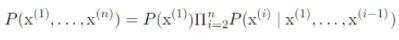
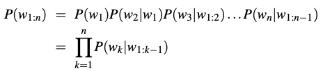
Using the definition of conditional probabilities, the decomposition (the joint probability of an entire sequence of words) using the chain rule of probability:

The intuition of the n-gram model is that instead of computing the probability of a word given its entire history, we can approximate the history by just the last few words.

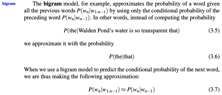
The assumption that the probability of a word depends only on the previous word is called a Markov assumption. Markov models are the class of probabilistic models that assume we can predict the probability of some future unit without looking too far into the past. We can generalize the bigram (which looks one word into the past) to the trigram (which looks two words into the past) and thus to the n-gram (which looks n − 1 words into the past).

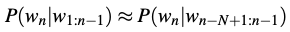
General equation for this n-gram approximation to the conditional probability of the next word in a sequence. We’ll use N here to mean the n-gram size, so N = 2 means bigrams and N = 3 means trigrams. Then we approximate the probability of a word given its entire context as follows:

To estimate probabilities, we use maximum likelihood estimation or MLE. For the general case of MLE n-gram parameter estimation:

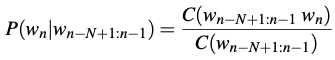
where $C(w_{n-N+1:n-1}w_n)$ is the count of the n-gram $w_{n-N+1:n-1}w_n$,
and $C(w_{n-N+1:n-1})$ is the sum of all the n-gram that start with a given word $w_{n-N+1:n-1}$ = the sum of all n-gram counts that start with a given word $w_{n-N+1:n-1}$ must be equal to the unigram count for that word $w_{n-N+1:n-1}$.

=> Equation estimates the n-gram probability by dividing the observed frequency of a particular sequence by the observed frequency of a prefix.
This ratio is called a relative frequency.

We always represent and compute language model probabilities in log format as log probabilities. Because:
1. Since probabilities are (by definition) less than or equal to 1, the more probabilities we multiply together, the smaller the product becomes.
2. Adding in log space is equivalent to multiplying in linear space, so we combine log probabilities by adding them.

Knerser-Ney Smoothing

---

2. Smoothing methods

2.1. Multinomial distribution and maximum likelihood estimation

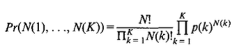
Here, we will use the term event or event class to describe the type of observations we are considering. When we are looking at word bigrams, the events will be the possible word pairs. In discussing conditional bigram probabilities for a fixed predecessor word, the events wil be the single words that may follow the fixed predecessor word.

Let us denote

• the event classes under consideration by $k=1,..., K$,
• their sample counts by $N(k)$, i.e. the frequency how often class $k$ was observed in the training text,
• the corresponding probabilities by $p(k)$, i.e. the chance of success of class $K$.

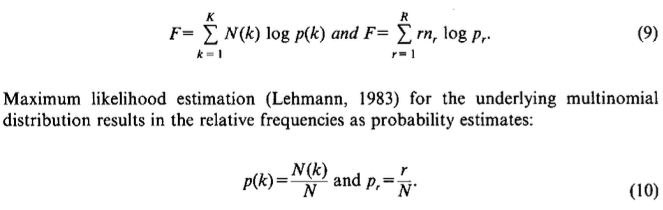
For a set of $N$ observations (in training or testing), we have $N$ independent trials with $K$ possible outcomes, where the sample counts $N(k)$ denote the number of trials resulting in class or outcome $k$. The distribution of the sample counts $N(k)$ is referred to as multinomial (or polynomial) distribution (Lehmann, 1983):

As we will see later, it is helpful to partition the event classes $k$ into equivalence classes according to their sample counts $r = N(k)$ (Good, 1953), which is referred to as symmetry requirement (Nadas, 1985). Let $n$, be the number of event classes which occured in the training text exactly r times and $p_r>0$ be the corresponding probability, i.e. we define:

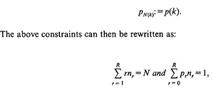
where we have: $n_r=0$ for $r>R$.

$F$ in terms of the sample counts $N(k)$ and of the equivalence class counts $n_r$:

2.2. Floor method and linear interpolation

To guarantee non-zero probability estimates, we can modify the sample counts N(k) by adding a floor value which is chosen proportional to probabilities q(k) of a less specific distribution, e.g. unigram distribution or uniform distribution. After renormalization, we then obtain the probability estimates:

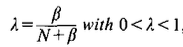
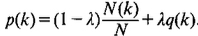
-> linear interpolation (each sample count $N(k)$ is reduced("discounted") by a value ${lamda}*N(k)$. However, it can be argued that the higher the sample counts $N(k)$, the higher their contribution should be in the interpolation model.

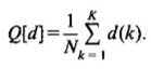
2.4 Discounting models

We introduce a general discounting function $d:k→ d(k)$ that has to be subtracted from every sample count N(k) and obtain the following smoothing formula:

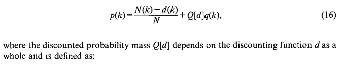
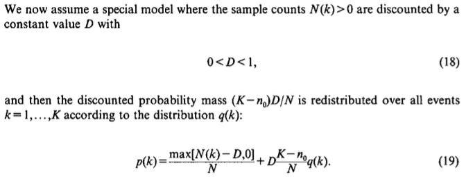
A constant value D with the range constraint0<D<1 can be intuitively interpreted as a correction that lies well within the range of the "discretization noise" of the discrete counts N(k). This nonlinear interpolation model has the following properties:

• The weight of the more general distribution q(k) is proportional to (K-n_0), which is the total number of different events k that were observed. This property is particularly attractive for modelling conditional probabilities: if a given word predecessor is followed by only one or a few different words, the smoothing effect will be much smaller than in the case where it is followed by many different words.
• Seting D=1 amounts to pooling al singletons, i.e. events k with N(k) =1, with the unseen events. As Katz (Katz, 1987) pointed out in asimilar context, there si not much difference between seeing an event just once or not at all.
• Although the interpolation is nonlinear, there is always a smoothing effect in that a weighted average between the two distributions is computed. This is different from Katz's backing-off approach (Katz, 1987), where a choice must be made between the more specific and the more general distribution.