[Paper Review] RNN + Long Short-Term Memory

6X10·2024년 4월 13일

NLP

목록 보기

2/3

Before the beginning,,,

What is Recurrent Neural Networks (RNN)?

RNNs use the idea of processing sequential information. The term “recurrent” applies as they perform the same task over each instance of the sequence such that the output is dependent on the previous computations and results. Generally, a fixed-size vector is produced to represent a sequence by feeding tokens one by one to a recurrent unit. In a way, RNNs have “memory” over previous computations and use this information in current processing.

Structure of Simple RNN

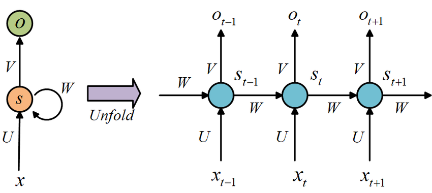
$x_t$ : the input to the network at time step $t$
$s_t$ : the hidden state at time step $t$

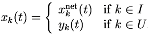
Caculation of $s_t$ is based as per the equation:

-> $s_t$ is caculated based on the current input and the previous time step's hidden state
-> $s_t$ is considered as the network’s memory element that accumulates information from other time steps

The function $f$ : a non-linear transformation such as $tanh, ReLU$
$U, V, W$ : weights that are shared across time

Properties of RNN
- Pros
  - Given that an RNN performs sequential processing by modeling units in sequence, it has the ability to capture the inherent sequential nature present in language, where units are characters, words or even sentences.
  - RNNs have flexible computational steps that provide better modeling capability and create the possibility to capture unbounded context.
- Cons
  - Simple RNN networks suffer from the infamous vanishing gradient problem, which makes it really hard to learn and tune the parameters of the earlier layers in the network.

Conventional BPTT (e.g., Williams and Zipser 1992)

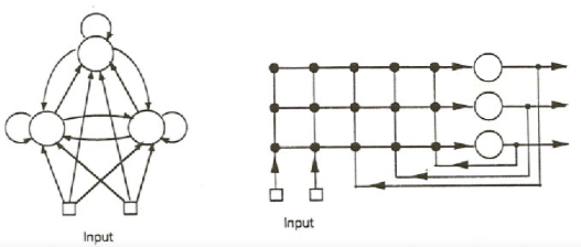
Network Architecture
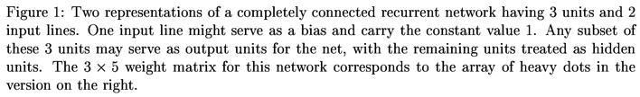
- Let the network have $n$ units, with $m$ external input lines.
- Let $y(t)$ denote the $n$ -tuple of outputs of the units in the network at time $t$ .
- Let $x^{net}(t)$ denote the $m$ -tuple of external input signals to the network at time t.
- We also define $x(t)$ to be the $(m+ n)$ -tuple obtained by concatenating $x^{net}(t)$ and $y(t)$ in some convenient fashion.
- Let $U$ denote the set of indices $k$ such that $x_k$ the $k^{th}$ component of $x$ , is the output of a unit in the network.
- Let $I$ denote the set of indices $k$ for which $x_k$ is an external input.
- Furthermore, we assume that the indices on $y$ and $x^{net}$ are chosen to correspond to those of x, so that
- Let $W$ denote the weight matrix for the network, with a unique weight between every pair of units and also from each input line to each unit.
- The element $w_{ij}$ represents the weight on the connection to the $i^{th}$ unit from either the $j^{th}$ unit, if $j \in U$ , or the $j^{th}$ input line, if $j \in I$ .
- Furthermore, note that to accommodate a bias for each unit we simply include among the $m$ input lines one input whose value is always 1; the corresponding column of the weight matrix contains as its $i^{th}$ element the bias for unit $i$ . In general, our naming convention dictates that we regard the weight $w_{ij}$ as having $x_j$ as its “presynaptic” signal and $y_j$ as its “postsynaptic” signal.
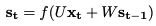
- For each k, the intermediate variable $s_{k}(t)$ represents the net input to the $k^{th}$ unit at time $t$ . Its value at time $t+1$ is computed in terms of both the state of and input to the network at time $t$ by
  
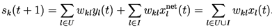
  The longer one clarifies how the unit outputs and the external inputs are both used in the computation, while the more compact expression illustrates why we introduced $x$ and the corresponding indexing convention above.
- The output of such a unit at time $t+1$ is then expressed in terms of the net input by
  
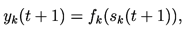
  where $f_k$ is the unit's squashing function.
- In those cases where a specific assumption (differentiable) about these squashing functions is required, it will be assumed that all units use the logistic function.
Network Performance Measure
- Assume that the task to be performed by the network is a sequential supervised learning task, meaning that certain of the units’ output values are to match specified target values (which we also call teacher signals) at specified times.
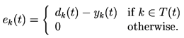
- Let $T(t)$ denote the set of indices $k \in U$ for which there exists a specified target value $d_k(t)$ that the output of the $k^{th}$ unit should match at time $t$ . Then define a time-varying $n$ -tuple $e$ by
  -> Note that this formulation allows for the possibility that target values are specified for different units at different times.
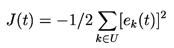
- Denote the negative of the overall network error at time t.
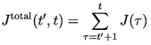
- A natural objective of learning might be to maximize the negative of the total error oversome appropriate time period $(t',t]$ .
- One natural wat to make the weight changes is along a constant positive multiple of the performance measure gradient, so that
  
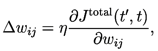
  for each $i$ and $j$ , where $\eta$ is a positive learning rate parameter.

LSTM

1. Introduction

With conventional "Back-Propagation Through Time" (BPTT) or "Real-Time Recurrent Learning" (RTRL), error signals "flowing backwards in time" tend to either (1) blow up or (2) vanish
(BPTT 참고: https://velog.io/@jody1188/BPTT)
-> LSTM is designed to overcome these error back-flow problems. It can learn to bridge time intervals in excess of 1000 steps even in case of noisy, incompressible input sequences, without loss of short time lag capabilities.

3. Constant Error Backprop

3.1 Exponentially Decaying Error

3.2 Constant Error Flow: NAIVE APPROACH

A single unit
- To avoid vanishing error signals, at time $t$ , $j$ 's local error back flow is
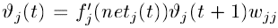
- To enfore constant error flow through $j$ , we require
The constant error carrousel
- Interating the differential equation above, we obtain
- This means: $f_j$ has to be linear, and unit $j$ 's activation has to remain constant:
- In the experiments, this will be ensured by using the identity function $f_j$ : $f_j(x)=x, \forall x$ , and by setting $w_{jj}=1.0$ . We refer to this as the constant error carrousel (CEC).

4. LONG SHORT-TERM MEMORY

Memory cells and gate units
- To construct an architecture that allows for constant error flow through special, self-connected units without the disadvantages of the naive approach, we extend the constant error carrousel CEC embodied by the self-connected, linear unit $j$ from Section 3.2 by introducin additional features.
- A multiplicative $input$ $gate$ $unit$ is introduced to protect the momory contents stored in $j$ from pertubation by irrelevant inputs. Likewise, a multiplicative $output$ $gate$ $unit$ is introduced which protects other units from perturbation by currently irrelevant memory contents stored in $j$ .